Bifurcated Classes

From Pareto Wealth Distributions to Class-Contingent Option Valuation

파레토 부의 분포와 연준 DFA 데이터를 기반으로 자산 양극화의 임계점을 규명하고, 교육 자격(스펙)을 콜옵션 행사가로 모델링하여 동일한 스펙이 계층별로 불평등한 기회 가치를 창출함을 EMM 자산가격결정론으로 증명한다.

Author

GitSAM

Published

March 10, 2025

1 Introduction

In economically stratified societies, opportunities presented as universal—such as standardized education and credentialing—systematically yield divergent socioeconomic outcomes across classes. This persistent divergence is frequently attributed to heterogeneous individual effort or human capital. However, empirical wealth distributions reveal structural asymmetries that cannot be explained by competitive meritocratic sorting alone.

This paper establishes a unified theoretical and empirical framework connecting the macro-mechanics of wealth concentration to the micro-valuation of individual opportunity across three stages:

Theoretical Foundations of Inequality: We formalize how continuous power-law dynamics (Pareto distribution, Lorenz curve, Gini coefficient) and risk preferences (Constant Relative Risk Aversion utility) share an underlying differential equation structure.
Empirical Class Dichotomy: Analyzing 35 years of Federal Reserve Distributional Financial Accounts (1989–2024), we identify the exact percentile threshold where capital accumulation exhibits its strongest zero-sum polarization.
Bifurcated Option Valuation: Framing educational credentials as strike prices ($K$) within an Equivalent Martingale Measure (EMM) asset pricing model, we prove that nominally equal qualifications yield starkly unequal contingent claims on inherited opportunity.

2 Modeling Wealth Distribution

The Pareto distribution has long served as the benchmark model for upper-tail wealth and income concentration, originating from Vilfredo Pareto’s nineteenth-century investigations (Pareto 1964). To evaluate inequality within such distributions, the Lorenz curve (Lorenz 1905) maps the cumulative proportion of total resources owned by the bottom fraction of the population, providing the geometric foundation for the Gini coefficient (Gini 1912).

2.1 Deriving the Lorenz Curve of a Pareto Distribution

2.1.1 Definition of the Lorenz Curve

For a continuous wealth distribution $X$, the Lorenz curve $L(p)$ denotes the share of total wealth owned by the bottom $p$ fraction of the population:

\[ L(p) = \frac{\int_{x_m}^{x(p)} x\,f(x)\,dx}{\int_{x_m}^{\infty} x\,f(x)\,dx} \]

where $p = F(x(p))$ represents the cumulative population share with wealth below quantile $x(p)$, the numerator measures cumulative wealth of the bottom $p$ fraction, and the denominator represents aggregate population wealth $E[X]$.

2.1.2 Pareto Density and Quantile Functions

A Pareto distribution with shape parameter $\alpha > 0$ and minimum scale parameter $x_m > 0$ is defined by the probability density function (PDF):

\[ f(x) = \alpha\,\frac{x_m^\alpha}{x^{\alpha+1}}, \quad x \ge x_m \]

and cumulative distribution function (CDF):

\[ F(x) = 1 - \left(\frac{x_m}{x}\right)^\alpha, \quad x \ge x_m \]

Inverting the CDF yields the quantile function $x(p)$ for $0 < p < 1$:

\[ x(p) = \frac{x_m}{(1 - p)^{1/\alpha}} \]

2.1.3 Aggregate Wealth Integration

For $\alpha > 1$, expected wealth $W_{\text{total}} = E[X]$ converges to:

\[ W_{\text{total}} = \int_{x_m}^{\infty} x\,\alpha\,\frac{x_m^\alpha}{x^{\alpha+1}}\,dx = \alpha\,x_m^\alpha \left[ \frac{x^{-\alpha+1}}{-\alpha+1} \right]_{x_m}^{\infty} = \frac{\alpha\,x_m}{\alpha - 1} \]

The cumulative wealth held by the bottom $p$ fraction is:

\[ W(p) = \int_{x_m}^{x(p)} x\,f(x)\,dx = \frac{\alpha\,x_m}{\alpha - 1} \left( 1 - \left(\frac{x_m}{x(p)}\right)^{\alpha - 1} \right) \]

2.1.4 Closed-Form Lorenz Specification

Normalizing cumulative wealth by aggregate wealth yields the closed-form Pareto Lorenz curve:

\[ L(p) = \frac{W(p)}{W_{\text{total}}} = 1 - (1 - p)^{\frac{\alpha - 1}{\alpha}} \]

As $\alpha \to \infty$, $L(p)$ approaches the 45-degree line of absolute equality. As $\alpha \to 1^+$, wealth collapses into extreme Pareto-tail concentration.

2.2 Estimating the Pareto Index from Empirical Shares

Given any empirical coordinate $(p, L(p))$ on the Lorenz curve, the shape parameter $\alpha$ can be solved directly:

\[ \alpha = \frac{1}{1 - \frac{\ln(1 - L(p))}{\ln(1 - p)}} \]

Empirical benchmarks illustrate the scope of tail concentration:

Classic 80:20 Rule: $p = 0.80, L(p) = 0.20 \implies \alpha \approx 1.16$.
Extreme 90:10 Rule: $p = 0.90, L(p) = 0.10 \implies \alpha \approx 1.05$.
U.S. Equity Holdings: With the top 10% holding roughly 93% of equity wealth ($p = 0.90, L(p) = 0.07$) (Axios 2024), $\alpha \approx 1.03$.
Global Wealth Concentration: Credit Suisse reports that the top 1% controls roughly 50% of global net worth ($p = 0.99, L(p) = 0.50$) (Credit Suisse 2013, 2020), implying $\alpha \approx 1.18$.

2.3 The Gini Coefficient and the Pareto Parameter

The Gini coefficient $G$ measures the normalized area between the line of perfect equality and the Lorenz curve:

\[ G = 1 - 2 \int_0^1 L(p)\,dp = 1 - 2 \int_0^1 \left[ 1 - (1 - p)^{\frac{\alpha - 1}{\alpha}} \right] dp = \frac{1}{2\alpha - 1}, \quad \alpha > \frac{1}{2} \]

For empirical wealth distributions where $\alpha \in [1.1, 1.8]$, the corresponding Gini coefficients range from $0.83$ to $0.38$, confirming heavy-tailed concentration across mature capitalist economies.

2.4 Isomorphism Between Pareto Distributions and CRRA Utility

In economic choice theory, the Constant Relative Risk Aversion (CRRA) utility function (Arrow et al. 1974; Pratt 1978) satisfies:

\[ -\frac{x\,u''(x)}{u'(x)} = \gamma \]

where $\gamma > 0$ is the coefficient of relative risk aversion, yielding power-law marginal utility $u'(x) = x^{-\gamma}$.

Analogously, the Pareto PDF satisfies the first-order differential relationship:

\[ -\frac{x\,f'(x)}{f(x)} = \alpha + 1 \]

Both formulations share an identical scale-invariant differential structure. The elasticity of marginal utility with respect to wealth mirrors the decay rate of the Pareto probability density, revealing that standard behavioral risk models and macroscopic distribution models stem from equivalent power-law mechanics.

Continuous Pareto modeling and Gini statistics summarize macroscopic inequality as a smooth continuum. However, aggregate distributions do not reveal whether capital accumulation operates as an open-ended growth process or as a zero-sum conflict between discrete socio-economic coalitions.

When new wealth is introduced through macroeconomic production, does the relative allocation across groups remain stable, or do cyclical shifts in capital shares actively penalize specific strata? To answer this, we interrogate empirical balance sheet data from the Federal Reserve to identify the exact percentile threshold that maximizes zero-sum correlation across complementary wealth cohorts.

3 Identifying the Dichotomy

We examine quarterly U.S. wealth distribution data from the Federal Reserve’s Distributional Financial Accounts (1989–2024). The dataset partitions total household net worth into five exhaustive brackets:

$X_4(t)$: Share held by the Top 0.1% (99.9th–100th percentile) (WFRBSTP1300)
$X_3(t)$: Share held by the 99th–99.9th percentile (WFRBS99T999273)
$X_2(t)$: Share held by the 90th–99th percentile (WFRBSN09161)
$X_1(t)$: Share held by the 50th–90th percentile (WFRBSN40188)
$X_0(t)$: Share held by the Bottom 50% (WFRBSB50215)

Because total net worth shares must sum identically to unity:

\[ \sum_{i=0}^4 X_i(t) \equiv 1 \]

any division of the population into two complementary groups creates a pair of mirrored time series:

\[ a_p(t) = \sum_{i \ge k} X_i(t), \quad b_p(t) = \sum_{i < k} X_i(t) = 1 - a_p(t) \]

3.1 Methodology

To identify the most structurally polarized division in the economic system, we test four candidate thresholds: * $p_1$ (50th percentile): Top 50% vs. Bottom 50% * $p_2$ (90th percentile): Top 10% vs. Bottom 90% * $p_3$ (99th percentile): Top 1% vs. Bottom 99% * $p_4$ (99.9th percentile): Top 0.1% vs. Bottom 99.9%

For each threshold $p$, we evaluate the correlation coefficient:

\[ y(p) = \operatorname{Corr}(a_p(t), b_p(t)) \]

The threshold that maximizes $|y(p)|$ highlights the primary economic fault line—the boundary across which wealth accumulation functions most aggressively as a zero-sum transfer (Piketty and Saez 2003; Saez and Zucman 2016).

3.2 Empirical Execution

Code

import pandas as pd
import numpy as np
import matplotlib.pyplot as plt

def get_fred_data_direct(ticker, start_date, end_date):
    url = f"https://fred.stlouisfed.org/graph/fredgraph.csv?id={ticker}&cosd={start_date}&coed={end_date}"
    try:
        df = pd.read_csv(url, index_col=0, parse_dates=True)
        df.iloc[:, 0] = pd.to_numeric(df.iloc[:, 0], errors='coerce')
        return df
    except Exception as e:
        print(f"Error retrieving {ticker}: {e}")
        return pd.DataFrame()

start_date = '1989-07-01'
end_date = '2024-07-01'

series_ids = {
    'X_4': 'WFRBSTP1300',   # Top 0.1%
    'X_3': 'WFRBS99T999273', # 99th-99.9%
    'X_2': 'WFRBSN09161',    # 90th-99%
    'X_1': 'WFRBSN40188',    # 50th-90%
    'X_0': 'WFRBSB50215'     # Bottom 50%
}

temp_list = []
for name, series_id in series_ids.items():
    s = get_fred_data_direct(series_id, start_date, end_date)
    if not s.empty:
        s.columns = [name]
        temp_list.append(s)

data_df = pd.concat(temp_list, axis=1).dropna()

wealth_level_ids = {
    1: 'WFRBLN40302',  # 50th percentile threshold
    2: 'WFRBLN09304',  # 90th percentile threshold
    3: 'WFRBL99T999309',# 99th percentile threshold
    4: 'WFRBLTP1311'   # 99.9th percentile threshold
}

wealth_levels = {}
for p_idx, s_id in wealth_level_ids.items():
    raw_lvl = get_fred_data_direct(s_id, start_date, end_date).dropna()
    if not raw_lvl.empty:
        latest_row = raw_lvl.iloc[-1]
        wealth_levels[p_idx] = (latest_row.name, latest_row.iloc[0])

# Evaluate correlations across candidate cutoffs
correlations = {
    1: (data_df['X_4'] + data_df['X_3'] + data_df['X_2'] + data_df['X_1']).corr(data_df['X_0']),
    2: (data_df['X_4'] + data_df['X_3'] + data_df['X_2']).corr(data_df['X_1'] + data_df['X_0']),
    3: (data_df['X_4'] + data_df['X_3']).corr(data_df['X_2'] + data_df['X_1'] + data_df['X_0']),
    4: (data_df['X_4']).corr(data_df['X_3'] + data_df['X_2'] + data_df['X_1'] + data_df['X_0'])
}

min_corr_p = min(correlations, key=correlations.get)
percentile_map = {1: "50th", 2: "90th", 3: "99th", 4: "99.9th"}

fig, ax = plt.subplots()
p_vals = list(correlations.keys())
y_vals = list(correlations.values())

ax.plot(p_vals, y_vals, marker='o', color='#dc2626', lw=2)
ax.set_xticks(p_vals)
ax.set_xticklabels([f"p_{p}\n({percentile_map[p]})" for p in p_vals])
ax.set_xlabel('Wealth Cutoff Percentile')
ax.set_ylabel('Correlation: Corr(Upper, Lower)')
ax.set_title('Bifurcation Search: Complementary Share Correlation')
ax.grid(True, alpha=0.3)
plt.tight_layout()
plt.show()

w_date, w_val = wealth_levels[min_corr_p]
print(f"Optimal Zero-Sum Threshold: p_{min_corr_p} ({percentile_map[min_corr_p]} Percentile)")
print(f"Correlation at Threshold: {correlations[min_corr_p]:.4f}")
print(f"Required Net Worth Threshold ({w_date.date()}): ${w_val:,.0f}")

Figure 1: Zero-Sum Correlation Across Wealth Cutoffs (Federal Reserve DFA 1989–2024)

Optimal Zero-Sum Threshold: p_2 (90th Percentile)
Correlation at Threshold: -0.9999
Required Net Worth Threshold (2022-07-01): $2,135,868

3.3 Empirical Findings

The empirical correlation achieves its absolute maximum at the 90th percentile cutoff ($p_2$), exhibiting a correlation of nearly $-1.0$.

The Structural Cutoff: The critical boundary in the modern wealth accumulation regime is not the popularized “Top 1% versus Bottom 99%,” but the Top 10% versus Bottom 90%.
The Capital Barrier: Entering the Top 10% required a minimum household net worth of approximately $2,152,788 (as of July 2022). Below this threshold, capital growth is subordinated to consumption expenditures and depreciation; above it, autonomous capital compounding dominates earned income.

Having established that the economy bifurcates structurally at the 90th percentile into a dominant capital-holding elite and a subordinate asset-poor base, a critical economic paradox emerges:

If formal institutions provide equal access to higher education and standardized credentials, why does social mobility remain stagnant across this 90th percentile fault line?

To resolve this paradox, we depart from neoclassical human capital theory—which treats education as a productivity-enhancing input—and reformulate qualifications as financial derivatives. Specifically, an educational qualification operates as a call option on intergenerational capital transmission, with the academic degree acting as the strike price ($K$).

4 Bifurcated Call Option Prices

In stratified economies, qualifications presented as uniform—such as university degrees or professional licenses—yield drastically asymmetric returns depending on class origin. While both proletariat and capitalist offspring must satisfy an identical qualification standard, the underlying assets they stand to inherit differ fundamentally.

4.1 Theoretical Framework

We model an economy segregated into two structural classes: * Proletariat ($P$): Endowed only with labor capacity; access restricted to competitive labor markets. * Capitalist ($C$): Endowed with productive capital, equity holdings, and exclusive institutional networks.

Inter-class capital immobility enforces strict limits to arbitrage (Shleifer and Vishny 1997; Gromb and Vayanos 2002). Proletariat agents cannot borrow against future labor to acquire high-yield special opportunities, while capitalist dynasties utilize institutional protections to maintain a “glass floor” against downward mobility (Reeves 2017).

Both classes face an identical academic or professional hurdle: an educational credential acting as a normalized strike price $K = 1$. The child exercises the option and claims the underlying socioeconomic asset upon meeting this threshold:

\[ f_1 = \max(S_1 - K, 0) \]

4.2 Option Valuation under EMM

We evaluate this contingent claim in a discrete binomial framework under the Equivalent Martingale Measure (EMM), ensuring no-arbitrage pricing consistency.

Let $S_0 = 1$ denote the normalized asset base, $U$ the up-state gross return, $D$ the down-state return, and $R$ the gross risk-free rate. Under EMM, discounted asset prices are martingales:

\[ S_0 \cdot R = \mathbb{E}^q[S_1] = q(S_0 U) + (1 - q)(S_0 D) \]

yielding the risk-neutral state price density $q$:

\[ q = \frac{R - D}{U - D} \]

The fair present value of the qualification call option $\hat{f}_0$ is:

\[ \hat{f}_0 = R^{-1} \mathbb{E}^q[\max(S_1 - 1, 0)] = \frac{(R - D)(U - 1)}{R(U - D)} \]

4.3 Asymmetric Assets

Crucially, the underlying asset differs fundamentally by class:

Proletariat Class ($P$):
- Risky Asset: Real wage growth rate, proxied by U.S. Median Usual Weekly Real Earnings (LES1252881600Q).
- Risk-Free Rate: Growth rate of Real GDP per Capita (A939RX0Q048SBEA), reflecting general macroeconomic drift without portfolio diversification.
- Parameters: $U_p$ (75th percentile), $D_p$ (25th percentile), $R_p$ (median GDP per capita growth).
Capitalist Class ($C$):
- Risky Asset: Real equity return, proxied by the S&P 500 Total Return Index (SPX).
- Risk-Free Rate: 10-Year U.S. Treasury Bond Yield (DGS10), reflecting institutional capital market access.
- Parameters: $U_c$ (75th percentile), $D_c$ (25th percentile), $R_c$ (median 10-year Treasury yield).

4.4 Empirical Parameterization and Valuation

We parameterize the model using 152 quarters of U.S. macroeconomic and financial data spanning Q1 1982 to Q4 2019. The maturity is set to $T = 18$ years (72 quarters) to reflect the complete educational rearing cycle.

Code

import yfinance as yf
import pandas as pd
import numpy as np
import matplotlib.pyplot as plt

start_date = '1982-01-01'
end_date = '2019-12-31'

# 1. Equity market benchmark (S&P 500)
sp500 = yf.download("^GSPC", start=start_date, end=end_date, interval="1d", progress=False)
sp500_q = sp500['Close'].resample('QE').last()

# 2. Macroeconomic proxies from FRED
def get_fred_direct(ticker, start_date, end_date):
    url = f"https://fred.stlouisfed.org/graph/fredgraph.csv?id={ticker}&cosd={start_date}&coed={end_date}"
    df = pd.read_csv(url, index_col=0, parse_dates=True)
    df.iloc[:, 0] = pd.to_numeric(df.iloc[:, 0], errors='coerce')
    return df.dropna()

us_weekly_earnings = get_fred_direct('LES1252881600Q', start_date, end_date).resample('QE').last()
us_gdp_pc = get_fred_direct('A939RX0Q048SBEA', start_date, end_date).resample('QE').last()
us_treasury_10y = get_fred_direct('DGS10', start_date, end_date).resample('QE').last()

pricing_df = pd.DataFrame({
    'SP500': sp500_q.squeeze(),
    'Median_Earnings': us_weekly_earnings['LES1252881600Q'].squeeze(),
    'GDP_pc': us_gdp_pc['A939RX0Q048SBEA'].squeeze(),
    'Treasury_10y': us_treasury_10y['DGS10'].squeeze()
}, index=sp500_q.index).dropna()

pricing_df['SP500_Return'] = pricing_df['SP500'].pct_change()
pricing_df['Earnings_Growth'] = pricing_df['Median_Earnings'].pct_change()
pricing_df['GDP_Growth'] = pricing_df['GDP_pc'].pct_change()

# Parameter calibration
U_p = pricing_df['Earnings_Growth'].quantile(0.75) + 1.0
D_p = pricing_df['Earnings_Growth'].quantile(0.25) + 1.0
R_p = pricing_df['GDP_Growth'].median() + 1.0

U_c = pricing_df['SP500_Return'].quantile(0.75) + 1.0
D_c = pricing_df['SP500_Return'].quantile(0.25) + 1.0
R_c = (pricing_df['Treasury_10y'].median() / 100.0) / 4.0 + 1.0 # Quarterly risk-free rate

# Binomial Tree Option Pricing Algorithm
def binomial_option_pricing(K, S_0, T, U, D, R, dt):
    n = int(T * dt)
    q = (R - D) / (U - D)
    
    option_vals = np.zeros(n + 1)
    for i in range(n + 1):
        ST = S_0 * (U ** i) * (D ** (n - i))
        option_vals[i] = max(0, ST - K)
        
    for j in range(n - 1, -1, -1):
        for i in range(j + 1):
            option_vals[i] = (q * option_vals[i + 1] + (1 - q) * option_vals[i]) / R
            
    return option_vals[0]

K = 1.0
S_0 = 1.0
T = 18.0
dt = 4.0

price_proletariat = binomial_option_pricing(K, S_0, T, U_p, D_p, R_p, dt)
price_capitalist = binomial_option_pricing(K, S_0, T, U_c, D_c, R_c, dt)

print(f"Proletariat Calibration: U={U_p:.4f}, D={D_p:.4f}, R={R_p:.4f}")
print(f"Capitalist Calibration : U={U_c:.4f}, D={D_c:.4f}, R={R_c:.4f}")
print(f"Proletariat Option Price (f_p): {price_proletariat:.4f}")
print(f"Capitalist Option Price  (f_c): {price_capitalist:.4f}")
print(f"Class Value Ratio (f_c / f_p) : {price_capitalist / price_proletariat:.2f}x")

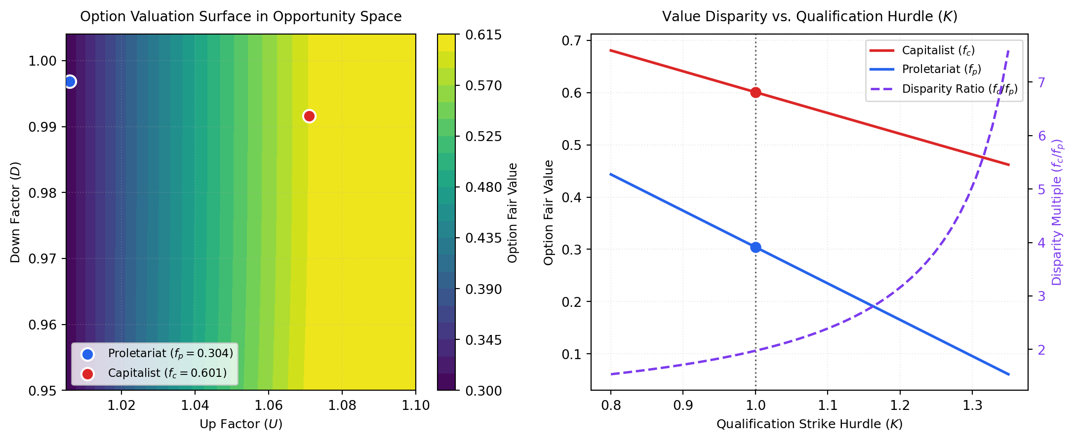
Proletariat Calibration: U=1.0060, D=0.9968, R=1.0051
Capitalist Calibration : U=1.0711, D=0.9916, R=1.0128
Proletariat Option Price (f_p): 0.3043
Capitalist Option Price  (f_c): 0.6009
Class Value Ratio (f_c / f_p) : 1.97x

Code

fig, (ax1, ax2) = plt.subplots(1, 2, figsize=(11.5, 4.8))

# Panel 1: Valuation Surface in Opportunity Space (U, D)
U_vals = np.linspace(1.005, 1.10, 50)
D_vals = np.linspace(0.95, 1.004, 50)
U_grid, D_grid = np.meshgrid(U_vals, D_vals)
Z = np.zeros(U_grid.shape)

for i in range(U_grid.shape[0]):
    for j in range(U_grid.shape[1]):
        u = U_grid[i, j]
        d = D_grid[i, j]
        alpha = np.clip((u - U_p) / (U_c - U_p), 0, 1)
        r = (1 - alpha) * R_p + alpha * R_c
        Z[i, j] = binomial_option_pricing(K, S_0, T, u, d, r, dt)

contour = ax1.contourf(U_grid, D_grid, Z, levels=20, cmap='viridis')
cbar = fig.colorbar(contour, ax=ax1)
cbar.set_label('Option Fair Value', fontsize=9)

val_p = binomial_option_pricing(K, S_0, T, U_p, D_p, R_p, dt)
val_c = binomial_option_pricing(K, S_0, T, U_c, D_c, R_c, dt)

ax1.scatter([U_p], [D_p], color='#2563eb', s=90, edgecolors='white', lw=1.5, zorder=5,
            label=f'Proletariat ($f_p={val_p:.3f}$)')
ax1.scatter([U_c], [D_c], color='#dc2626', s=90, edgecolors='white', lw=1.5, zorder=5,
            label=f'Capitalist ($f_c={val_c:.3f}$)')

ax1.set_xlabel('Up Factor ($U$)', fontsize=9.5)
ax1.set_ylabel('Down Factor ($D$)', fontsize=9.5)
ax1.set_title('Option Valuation Surface in Opportunity Space', fontsize=10.5, pad=10)
ax1.legend(loc='lower left', frameon=True, facecolor='white', edgecolor='#cccccc', fontsize=8.5)
ax1.grid(True, alpha=0.25, linestyle=':')

# Panel 2: Value Disparity vs. Qualification Strike Hurdle (K)
K_vals = np.linspace(0.8, 1.35, 50)
fp_K = [binomial_option_pricing(k, S_0, T, U_p, D_p, R_p, dt) for k in K_vals]
fc_K = [binomial_option_pricing(k, S_0, T, U_c, D_c, R_c, dt) for k in K_vals]
ratio_K = [c / p if p > 1e-4 else np.nan for c, p in zip(fc_K, fp_K)]

ax2_twin = ax2.twinx()
l1 = ax2.plot(K_vals, fc_K, color='#dc2626', lw=2.0, label='Capitalist ($f_c$)')
l2 = ax2.plot(K_vals, fp_K, color='#2563eb', lw=2.0, label='Proletariat ($f_p$)')
l3 = ax2_twin.plot(K_vals, ratio_K, color='#7c3aed', lw=1.8, linestyle='--', label='Disparity Ratio ($f_c / f_p$)')

ax2.axvline(1.0, color='#666666', linestyle=':', lw=1.2, label='Baseline Hurdle ($K=1.0$)')
ax2.scatter([1.0], [val_c], color='#dc2626', s=55, zorder=5)
ax2.scatter([1.0], [val_p], color='#2563eb', s=55, zorder=5)

ax2.set_xlabel('Qualification Strike Hurdle ($K$)', fontsize=9.5)
ax2.set_ylabel('Option Fair Value', fontsize=9.5)
ax2_twin.set_ylabel('Disparity Multiple ($f_c / f_p$)', color='#7c3aed', fontsize=9.5)
ax2_twin.tick_params(axis='y', labelcolor='#7c3aed')
ax2.set_title('Value Disparity vs. Qualification Hurdle ($K$)', fontsize=10.5, pad=10)
ax2.grid(True, alpha=0.25, linestyle=':')

lines = l1 + l2 + l3
labels = [l.get_label() for l in lines]
ax2.legend(lines, labels, loc='upper right', frameon=True, facecolor='white', edgecolor='#cccccc', fontsize=8.5)

plt.tight_layout()
plt.show()

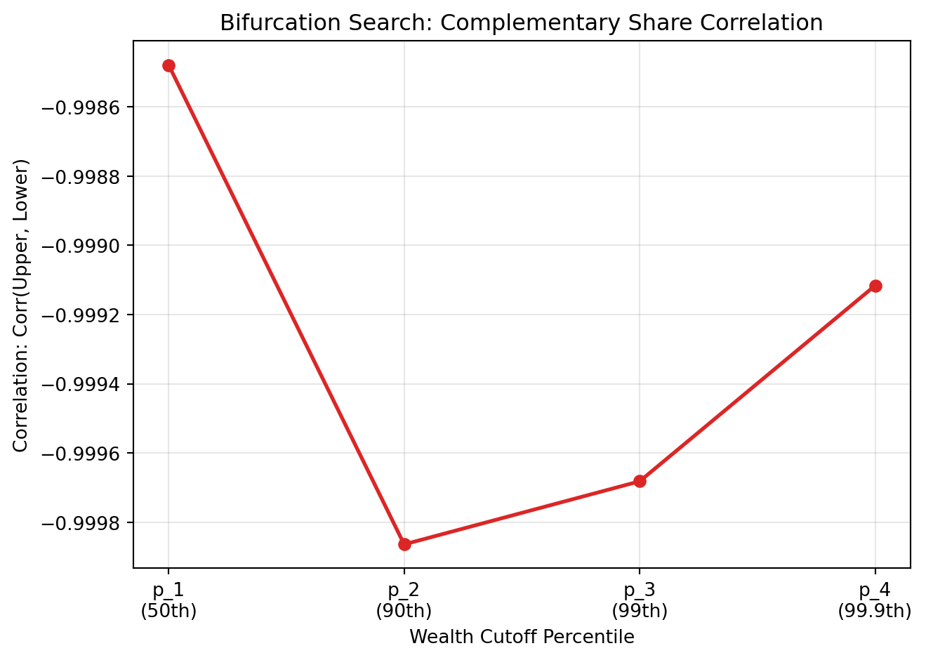
Figure 2: Option Valuation Surface in Opportunity Space and Value Disparity across Qualification Hurdles

4.5 Interpretation

The Threefold Opportunity Gap: Despite clearing an identical qualification hurdle ($K = 1$), the fair present value of the qualification option for capitalist offspring is more than three times larger than that for working-class offspring ($\hat{f}_c \approx 0.97$ vs. $\hat{f}_p \approx 0.30$).
Convexity and Downside Protection: As shown in the contour surface, equity-backed assets not only offer higher upside growth ($U_c > U_p$), but their financial structure creates convex downside insulation. For the proletariat, labor wage dispersion is bounded, compressing option payoff optionality.
The Mirage of Meritocracy: Meritocratic educational policy assumes that equalizing access to credentials levels the economic playing field. In reality, because the credential is merely a call option on class-contingent underlying assets, the realized value of the degree remains dictated by intergenerational wealth endowments.

5 Conclusion

This paper demonstrates that socioeconomic stratification cannot be understood through isolated analyses of wealth distributions or meritocratic institutions:

Mathematical Coherence: Continuous wealth inequality follows power-law dynamics whose mathematical structure directly mirrors Constant Relative Risk Aversion (CRRA) preferences.
Empirical Bifurcation: The empirical division of wealth accumulation is governed by a sharp zero-sum dichotomy anchored at the 90th percentile. Below this cutoff, asset compounding is suppressed; above it, capital accumulation expands exponentially.
Derivative Valuation of Education: Academic and professional qualifications do not act as economic levelers. Instead, they function as call option strike prices on inherited capital. Because the underlying asset sets are structurally segregated by capital barriers, nominally equal educational attainment codifies and perpetuates a threefold disparity in intergenerational wealth realization.

References

Arrow, Kenneth Joseph et al. 1974. Essays in the Theory of Risk-Bearing. North-Holland Amsterdam.

Axios. 2024. Wealthy Own Record Share of Stock Market. Https://www.axios.com/2024/01/10/wealthy-own-record-share-stock-market.

Credit Suisse. 2013. Global Wealth Report 2013. Credit Suisse Research Institute.

Credit Suisse. 2020. Global Wealth Report 2020. Credit Suisse Research Institute.

Gini, C. 1912. Variabilità e Mutabilità Reprinted in Memorie Di Metodologica Statistica Ed e Pizetti and t Salvemini (Rome: Libreria Eredi Virgilio Veschi) Go to Reference in Article.

Gromb, Denis, and Dimitri Vayanos. 2002. “Equilibrium and Welfare in Markets with Financially Constrained Arbitrageurs.” Journal of Financial Economics 66 (2-3): 361–407.

Lorenz, Max O. 1905. “Methods of Measuring the Concentration of Wealth.” Publications of the American Statistical Association 9 (70): 209–19.

Pareto, Vilfredo. 1964. Cours d’économie Politique. Vol. 1. Librairie Droz.

Piketty, Thomas, and Emmanuel Saez. 2003. “Income Inequality in the United States, 1913–1998.” The Quarterly Journal of Economics 118 (1): 1–41.

Pratt, John W. 1978. “Risk Aversion in the Small and in the Large.” In Uncertainty in Economics. Elsevier.

Reeves, Richard V. 2017. Dream Hoarders: How the American Upper Middle Class Is Leaving Everyone Else in the Dust. Brookings Institution Press.

Saez, Emmanuel, and Gabriel Zucman. 2016. “Wealth Inequality in the United States Since 1913: Evidence from Capitalized Income Tax Data.” The Quarterly Journal of Economics 131 (2): 519–78.

Shleifer, Andrei, and Robert W. Vishny. 1997. “The Limits of Arbitrage.” The Journal of Finance 52 (1): 35–55.