Labor–Capital Dynamics in AX

A Non-Equilibrium Perspective on Decoupling and Degeneracy

자동화(AX) 환경에서 노동과 자본의 비평형 동역학계를 구축하고, 연준 부의 분배 데이터(1989~2024)를 통해 자본의 자가증식과 노동 탈동조화(Decoupling)가 초래하는 체계적 불안정성 및 위상공간 붕괴 메커니즘을 분석한다.

Abstract

Automation is fundamentally altering the capital–labor relationship beyond neoclassical general equilibrium and Marxian surplus extraction. We develop a non-conservative dynamical system extending Goodwin-type interactions to capture autonomous capital compounding, elite-elite congestion rivalry (\(C^2\)), and labor decoupling. Calibrating the model on U.S. Federal Reserve Distributional Financial Accounts (1989–2024) across Top 0.1%, 1%, and 10% net wealth shares, we uncover an empirical regime where labor-driven capital accumulation drops to near zero (\(a_{21} \approx 0\)). We identify a critical structural paradox: complete decoupling leads to systemic collapse—extinguishing capital alongside labor—whereas an infinitesimal coupling (\(a_{21} = 0.0007\)) restores long-run persistence matching observed distributions. These findings demonstrate that economic stability and inequality are governed by phase-space geometry and feedback curvature rather than marginal productivity. Ethical system design must therefore prioritize anticipatory structural interventions over ex-post redistribution.

Keywords

automation, wealth inequality, nonlinear dynamics, replicator systems, predator-prey, capital-labor decoupling, elite rivalry, economic design

1 Introduction

Mainstream macroeconomic models predominantly treat capital and labor through the lens of static equilibrium, symmetric interaction, and marginal productivity theory (Acemoglu and Restrepo 2018; Andrew Berg and Zanna 2018). In these frameworks, technological change is formalized as an exogenous factor-augmenting shock that shifts factor demand while preserving structural co-dependence. Observed disparities in wealth and income are frequently rationalized as competitive reflections of heterogeneous talent or effort (Piketty 2014; Seth Benzell and Sachs 2015).

However, this meritocratic narrative commits a fundamental category error: while human physical and cognitive abilities are symmetrically distributed with thin tails, empirical wealth distributions across capitalist economies exhibit extreme Pareto-tail concentration. The primary driver of extreme inequality is not variance in individual input, but structural asymmetry in accumulation—driven by preferential attachment, winner-take-all mechanics, and institutional insulation. Elites operate in an environment where personal risk is minimized while systemic downside is socialized, turning formal competitive constraints into selective instruments.

Furthermore, the contemporary acceleration of automation, artificial intelligence, and algorithmic platforms (the AX era) invalidates the foundational assumption of factor co-dependence (Susskind 2020). Capital increasingly exhibits autopoietic reproduction—the capacity to compound, optimize, and allocate without human labor inputs. In classical political economy (Marx 1867) and heterodox macro-dynamics (Goodwin 1967; Flaschel 2009), capital accumulation inherently required the extraction or coordination of labor. When automation breaks this link, the dynamical system undergoes a qualitative mutation: the phase space ceases to be conservative, closed orbits vanish, and labor exclusion becomes a topologically absorbing state.

This paper formulates a compact, nonlinear dynamical system of labor (\(L\)) and capital (\(C\)) under automation, estimates its structural parameters using quarterly U.S. wealth share data (1989–2024), and demonstrates the paradoxical fragility of capital when completely severed from labor.

2 The Model

2.1 Classical Benchmark: Conservative Lotka–Volterra Cycles

To contextualize structural mutation, we first examine the canonical closed Lotka–Volterra baseline (Lotka 1925; Volterra 1926; Goodwin 1967). Here, prey \(L\) (labor) and predator \(C\) (capital) co-evolve under strict conservation of interaction energy:

\[ \begin{aligned} \dot{L} &= L (a_{11} - a_{12} C), \\ \dot{C} &= C (a_{21} L - a_{22}). \end{aligned} \]

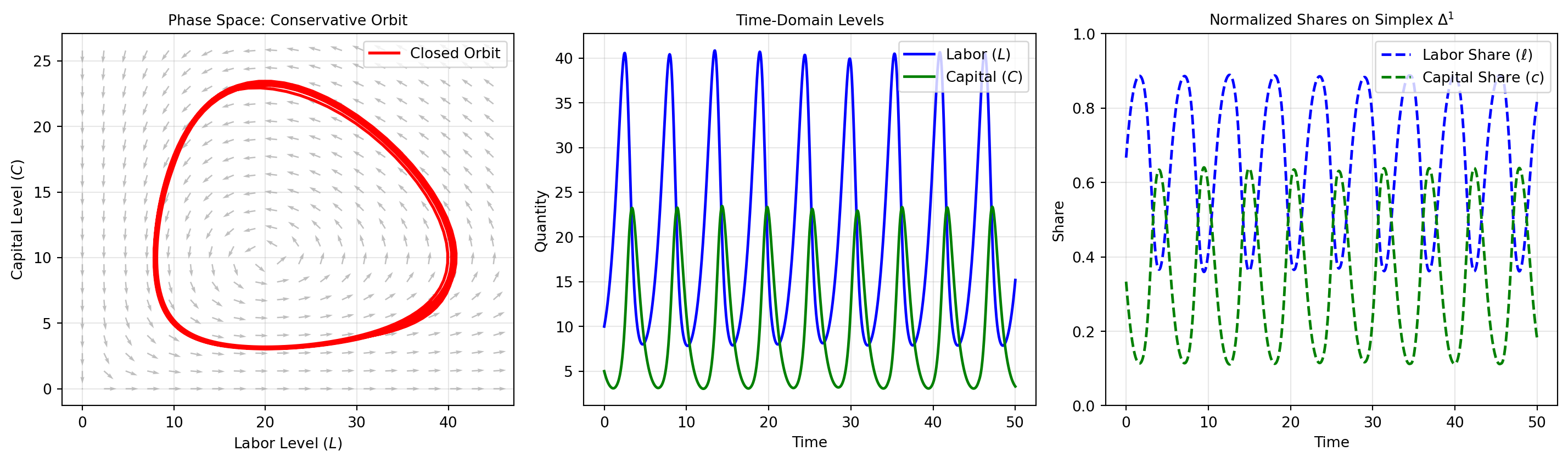
As illustrated in Figure 1, this system traces closed orbits in phase space without converging to an absorbing boundary or permitting species extinction. However, it cannot capture structural mutations, autopoietic capital self-replication, or labor-displacement regimes.

import numpy as np
import matplotlib.pyplot as plt
from scipy.integrate import solve_ivp

# Parameters for conservative predator-prey system
a11_c, a12_c = 1.0, 0.1
a21_c, a22_c = 0.075, 1.5

def lotka_volterra_classical(t, y):
    L, C = y
    dL = a11_c * L - a12_c * L * C
    dC = a21_c * L * C - a22_c * C
    return [dL, dC]

t_span = (0, 50)
t_eval = np.linspace(0, 50, 1000)
sol_c = solve_ivp(lotka_volterra_classical, t_span, [10.0, 5.0], t_eval=t_eval)
t_c, L_c, C_c = sol_c.t, sol_c.y[0], sol_c.y[1]

fig, (ax1, ax2, ax3) = plt.subplots(1, 3, figsize=(15, 4.5))

# 1. Phase space vector field & trajectory
L_max, C_max = max(L_c) * 1.1, max(C_c) * 1.1
L_grid, C_grid = np.meshgrid(np.linspace(0, L_max, 20), np.linspace(0, C_max, 20))
dL_grid = a11_c * L_grid - a12_c * L_grid * C_grid
dC_grid = a21_c * L_grid * C_grid - a22_c * C_grid
mag = np.sqrt(dL_grid**2 + dC_grid**2) + 1e-8

ax1.quiver(L_grid, C_grid, dL_grid/mag, dC_grid/mag, color='gray', alpha=0.5)
ax1.plot(L_c, C_c, 'r-', lw=2, label="Closed Orbit")
ax1.set_title("Phase Space: Conservative Orbit", fontsize=10)
ax1.set_xlabel("Labor Level $(L)$")
ax1.set_ylabel("Capital Level $(C)$")
ax1.grid(True, alpha=0.3)
ax1.legend()

# 2. Time domain levels
ax2.plot(t_c, L_c, 'b-', label="Labor $(L)$", lw=1.8)
ax2.plot(t_c, C_c, 'g-', label="Capital $(C)$", lw=1.8)
ax2.set_title("Time-Domain Levels", fontsize=10)
ax2.set_xlabel("Time")
ax2.set_ylabel("Quantity")
ax2.grid(True, alpha=0.3)
ax2.legend()

# 3. Normalized shares
l_share = L_c / (L_c + C_c)
c_share = C_c / (L_c + C_c)
ax3.plot(t_c, l_share, 'b--', label="Labor Share $(\\ell)$", lw=1.8)
ax3.plot(t_c, c_share, 'g--', label="Capital Share $(c)$", lw=1.8)
ax3.set_title("Normalized Shares on Simplex $\\Delta^1$", fontsize=10)
ax3.set_xlabel("Time")
ax3.set_ylabel("Share")
ax3.set_ylim(0, 1)
ax3.grid(True, alpha=0.3)
ax3.legend()

plt.tight_layout()
plt.show()

Figure 1: Classical Conservative Lotka–Volterra Benchmark: (A) Phase plane trajectory forming closed orbits; (B) Perpetual oscillation in population levels; (C) Normalized shares on the 1-simplex \(\Delta^1\).

2.2 Level-Based Dynamics with Autopoiesis and Elite Rivalry

To accommodate structural mutation, we formalize the co-evolution of aggregate labor \(L(t)\) and capital \(C(t)\) by extending the baseline into an open, asymmetric dynamical system:

\[ \begin{aligned} \frac{dL}{dt} &= a_{11} L - a_{12} L C, \\ \frac{dC}{dt} &= a_{21} L C + a_{22} C - a_{23} C - a_{24} C^2. \end{aligned} \]

The structural parameters govern precise economic mechanisms:

• \(a_{11} > 0\): Autonomous labor renewal rate (demographic reproduction, training, basic workforce entry).
• \(a_{12} > 0\): Capital-induced labor displacement (automation, skill obsolescence, capital substitution).
• \(a_{21} \ge 0\): Labor-mediated capital accumulation (traditional surplus generation through human labor).
• \(a_{22} \ge 0\): Autopoietic capital growth (AI self-replication, algorithmic scaling, compounding without labor).
• \(a_{23} > 0\): Capital depreciation and maintenance decay.
• \(a_{24} > 0\): Intra-elite congestion and saturation friction.

Unlike conventional neoclassical models where quadratic cost terms represent technological diminishing returns to scale, \(-a_{24} C^2\) here captures intra-elite positional rivalry. In a financialized economy saturated with capital, holders compete not against labor, but against rival capital blocks for scarce sovereign collateral, speculative rents, and regulatory capture. It reflects structural friction born of excessive concentration at the top.

2.3 Simplex Normalization and Replicator Dynamics

To analyze distribution invariant to system scale, we normalize levels onto the unit 1-simplex \(\Delta^1\). Defining total mass \(S(t) = L(t) + C(t)\), we express the system in relative shares:

\[ c(t) = \frac{C(t)}{S(t)}, \quad \ell(t) = \frac{L(t)}{S(t)} = 1 - c(t). \]

Differentiating \(c(t)\) with respect to time yields:

\[ \dot{c} = \frac{\dot{C}S - C\dot{S}}{S^2} = c(1 - c) \left[ \frac{\dot{C}}{C} - \frac{\dot{L}}{L} \right]. \]

Under structural decoupling where direct labor contribution to capital formation approaches zero (\(a_{21} \approx 0\)), and considering short-horizon quasi-stationarity of aggregate scale, the capital share dynamics simplifies to a canonical replicator equation:

\[ \frac{dc}{dt} \approx c(t) \left[ a_{22} - a_{24} c(t) \right]. \]

In discrete empirical observation windows, this maps directly to:

\[ \frac{\Delta c_t}{c_t} \approx a_{22}(t) - a_{24}(t) c_t. \]

Equation reveals that capital share evolution is dictated by the tension between automation compounding (\(a_{22}\)) and intra-elite positional saturation (\(a_{24}\)).

2.4 Asymptotic Regimes and Irreversibility

Depending on parameter configurations, the system displays distinct topological behaviors:

1. Classical Mutualism (\(a_{22} = 0, a_{21} > 0\)): Conservative Goodwin-style cyclical orbits around an interior fixed point. Capital and labor remain mutually bounded.
2. Structural Mutation (\(a_{22} > a_{23}, a_{21} \to 0\)): Capital growth uncouples from labor. Once \(a_{12} C > a_{11}\), labor experiences exponential decay toward the boundary \(L = 0\).
3. Topological Irreversibility: The subspace \(L = 0\) is an absorbing boundary. Once labor is excluded from phase space, internal vector fields provide no restorative trajectory.

3 Empirical Calibration: U.S. Top Wealth Shares (1989–2024)

3.1 Data and Estimation Strategy

We retrieve quarterly net wealth share data from the Federal Reserve’s Distributional Financial Accounts (DFA via FRED) covering 1989Q3 to 2024Q4:

• Top 0.1% Net Wealth Share (WFRBSTP1300)
• Top 1% Net Wealth Share (WFRBST01134)
• Top 10% Net Wealth Share (Sum of Top 1% and 90–99% WFRBSN09161)

import pandas as pd
import numpy as np
import matplotlib.pyplot as plt
from scipy.integrate import solve_ivp
from scipy.stats import trim_mean, mode

# 1. Direct fetch from FRED DFA
def get_fred_data_direct(ticker, start_date="1989-07-01", end_date="2024-10-01"):
    url = f"https://fred.stlouisfed.org/graph/fredgraph.csv?id={ticker}&cosd={start_date}&coed={end_date}"
    df_raw = pd.read_csv(url, index_col=0, parse_dates=True)
    df_raw.iloc[:, 0] = pd.to_numeric(df_raw.iloc[:, 0], errors='coerce')
    return df_raw.dropna()

tickers = {
    'Top 0.1%': 'WFRBSTP1300',
    'Top 1%': 'WFRBST01134',
    'Top 90-99%': 'WFRBSN09161'
}

raw_data = {lbl: get_fred_data_direct(tk) for lbl, tk in tickers.items()}
df_fred = pd.concat([raw_data['Top 0.1%'], raw_data['Top 1%'], raw_data['Top 90-99%']], axis=1)
df_fred.columns = ['Top_0.1', 'Top_1', 'Top_90_99']
df_fred['Top_10'] = df_fred['Top_1'] + df_fred['Top_90_99']
df = df_fred[['Top_0.1', 'Top_1', 'Top_10']].dropna()

df.head()

Table 1: Quarterly Net Wealth Share Samples from FRED DFA (Top 0.1%, 1%, and 10%).

	Top_0.1	Top_1	Top_10
observation_date
1989-07-01	8.6	22.8	60.8
1989-10-01	8.7	23.0	60.9
1990-01-01	8.6	22.8	60.5
1990-04-01	8.7	22.9	60.5
1990-07-01	8.4	22.4	59.8

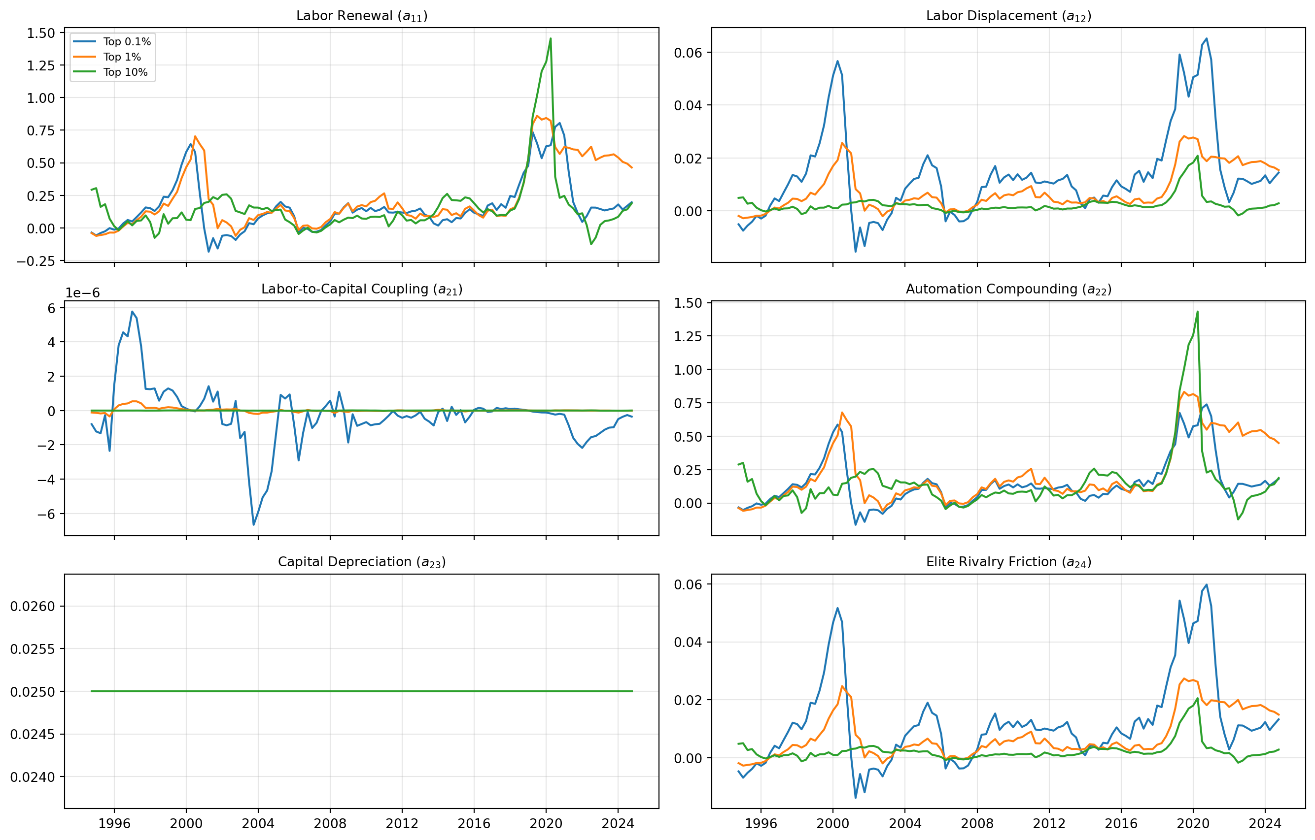
Using 20-quarter rolling OLS regressions on normalized growth rates, we estimate time-varying parameters \(a_{22}(t)\) and \(a_{24}(t)\) from capital share growth, \(a_{11}(t)\) and \(a_{12}(t)\) from labor share dynamics, and recover \(a_{21}(t)\) as the residual coupling coefficient under calibrated quarterly depreciation \(a_{23} = 0.025\).

ct_01 = df['Top_0.1']
ct_1 = df['Top_1']
ct_10 = df['Top_10']

# Rolling estimation function
def estimate_parameters(c_t, window=20, depreciation=0.025):
    c_t = c_t.dropna()
    l_t = 1.0 - c_t
    dc = c_t.diff()
    dl = l_t.diff()
    c_lag = c_t.shift(1)
    l_lag = l_t.shift(1)
    
    rel_dc = (dc / c_lag).dropna()
    rel_dl = (dl / l_lag).dropna()

    df_rolling = pd.DataFrame({
        'c': c_lag, 'l': l_lag,
        'dc_rel': rel_dc, 'dl_rel': rel_dl
    }).dropna()

    results = []
    for i in range(window, len(df_rolling)):
        win = df_rolling.iloc[i - window:i]
        
        # Capital equation: dc/c = a22 - a24*c
        Xc = np.vstack([np.ones(window), -win['c']]).T
        yc = win['dc_rel']
        a22, a24 = np.linalg.lstsq(Xc, yc, rcond=None)[0]

        # Labor equation: dl/l = a11 - a12*c
        Xl = np.vstack([np.ones(window), -win['c']]).T
        yl = win['dl_rel']
        a11, a12 = np.linalg.lstsq(Xl, yl, rcond=None)[0]

        # Residual coupling: a21
        residual_c = yc - (a22 - a24 * win['c'])
        a21 = np.mean(residual_c / win['l'])
        a23 = depreciation

        results.append({
            'date': df_rolling.index[i],
            'a11': a11, 'a12': a12, 'a21': a21,
            'a22': a22, 'a23': a23, 'a24': a24
        })

    return pd.DataFrame(results).set_index('date')

res_df_01 = estimate_parameters(ct_01, window=20)
res_df_1 = estimate_parameters(ct_1, window=20)
res_df_10 = estimate_parameters(ct_10, window=20)

# Plot rolling parameter estimates
group_labels = ['Top 0.1%', 'Top 1%', 'Top 10%']
results_list = [res_df_01, res_df_1, res_df_10]
params = ['a11', 'a12', 'a21', 'a22', 'a23', 'a24']
param_titles = [
    r'Labor Renewal ($a_{11}$)', r'Labor Displacement ($a_{12}$)',
    r'Labor-to-Capital Coupling ($a_{21}$)', r'Automation Compounding ($a_{22}$)',
    r'Capital Depreciation ($a_{23}$)', r'Elite Rivalry Friction ($a_{24}$)'
]

fig, axes = plt.subplots(3, 2, figsize=(14, 9), sharex=True)
axes = axes.flatten()

for i, param in enumerate(params):
    for group_df, label in zip(results_list, group_labels):
        if param in group_df.columns:
            axes[i].plot(group_df.index, group_df[param], label=label, lw=1.5)
    axes[i].set_title(param_titles[i], fontsize=10)
    axes[i].grid(True, alpha=0.3)
    if i == 0:
        axes[i].legend(loc='upper left', fontsize=8)

plt.tight_layout()
plt.show()

Figure 2: Estimated Time-Varying Parameters for Each Wealth Percentile Group (1994-2024). Each panel tracks one structural parameter across Top 0.1%, Top 1%, and Top 10% tiers.

fig, axes = plt.subplots(3, 2, figsize=(13, 8))
axes = axes.flatten()
colors = ['tab:blue', 'tab:orange', 'tab:green']

for i, param in enumerate(params):
    ax = axes[i]
    for group_df, label, col in zip(results_list, group_labels, colors):
        ax.hist(group_df[param].dropna(), bins=40, alpha=0.55, label=label, color=col)
    ax.set_title(param_titles[i], fontsize=10)
    ax.set_xlabel("Value")
    ax.set_ylabel("Frequency")
    ax.grid(True, alpha=0.3)
    if i == 0:
        ax.legend(fontsize=8)

plt.tight_layout()
plt.show()

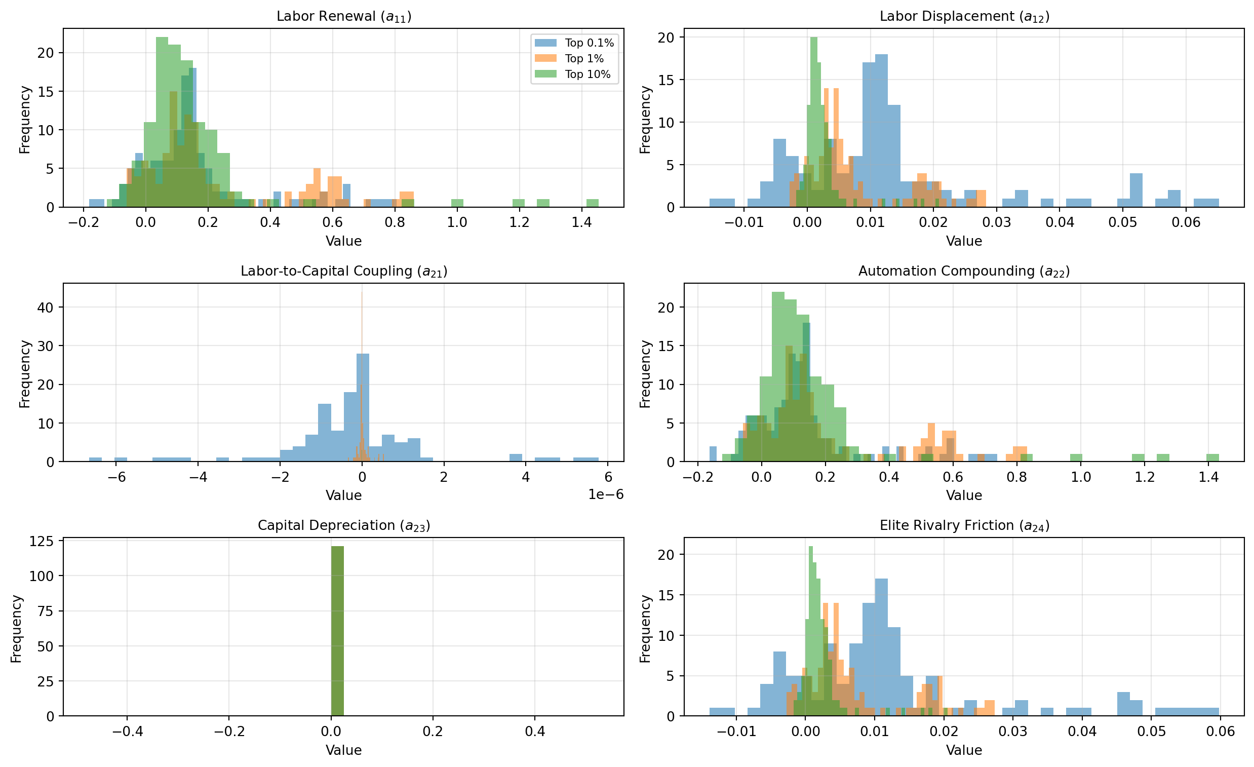
Figure 3: Empirical Distribution of Estimated Parameters Across Percentile Tiers. Visual comparison reveals structural dispersion across wealth classes.

3.2 Parameter Summary Statistics

depreciation = 0.025

def summarize_parameters(df_param, name):
    summary = pd.DataFrame(index=df_param.columns)
    summary["median"] = df_param.median()
    summary["trimmed_mean"] = df_param.apply(lambda x: trim_mean(x.dropna(), 0.1))
    summary["mode"] = df_param.mode().iloc[0]
    summary["group"] = name
    return summary

param_summary = pd.concat([
    summarize_parameters(res_df_01, "Top 0.1%"),
    summarize_parameters(res_df_1, "Top 1%"),
    summarize_parameters(res_df_10, "Top 10%")
]).reset_index().rename(columns={"index": "parameter"})

param_summary.loc[param_summary["parameter"] == "a23", ["median", "trimmed_mean", "mode"]] = depreciation

# Extract median parameter sets for simulation
def extract_params(df_summary, group_name):
    row = df_summary[df_summary["group"] == group_name].set_index("parameter")
    return {
        "a11": row.loc["a11", "median"],
        "a12": row.loc["a12", "median"],
        "a21": row.loc["a21", "median"],
        "a22": row.loc["a22", "median"],
        "a23": depreciation,
        "a24": row.loc["a24", "median"]
    }

params_top_01 = extract_params(param_summary, "Top 0.1%")
params_top_1 = extract_params(param_summary, "Top 1%")
params_top_10 = extract_params(param_summary, "Top 10%")

pivot_all = param_summary.pivot_table(
    index="parameter",
    columns="group",
    values=["median", "trimmed_mean", "mode"]
)

ordered_cols = [
    ("median", "Top 0.1%"), ("median", "Top 1%"), ("median", "Top 10%"),
    ("trimmed_mean", "Top 0.1%"), ("trimmed_mean", "Top 1%"), ("trimmed_mean", "Top 10%"),
    ("mode", "Top 0.1%"), ("mode", "Top 1%"), ("mode", "Top 10%"),
]
pivot_all = pivot_all[ordered_cols].round(5)
pivot_all

Table 2: Summary Statistics of Structural Parameters Across Elite Groups (Median, Trimmed Mean, Mode).

	median			trimmed_mean			mode
group	Top 0.1%	Top 1%	Top 10%	Top 0.1%	Top 1%	Top 10%	Top 0.1%	Top 1%	Top 10%
parameter
a11	0.12351	0.13422	0.10486	0.12756	0.19772	0.11464	-0.18211	-0.06067	-0.12472
a12	0.01074	0.00467	0.00153	0.01070	0.00679	0.00173	-0.01550	-0.00283	-0.00176
a21	-0.00000	-0.00000	-0.00000	-0.00000	0.00000	0.00000	-0.00001	-0.00000	-0.00000
a22	0.11208	0.12905	0.10337	0.11571	0.19068	0.11287	-0.16318	-0.05853	-0.12281
a23	0.02500	0.02500	0.02500	0.02500	0.02500	0.02500	0.02500	0.02500	0.02500
a24	0.00981	0.00450	0.00151	0.00970	0.00655	0.00170	-0.01388	-0.00273	-0.00173

3.3 Key Empirical Findings

1. Near-Zero Labor Coupling (\(a_{21} \to 0\)): Median empirical values of \(a_{21}(t)\) across all three wealth tiers are statistically negligible (\(< 10^{-5}\)), confirming that in late-stage financialized economies, elite wealth accumulation does not draw structural momentum from domestic labor input.
2. Structural Spikes in \(a_{22}(t)\): The autonomous compounding parameter rises markedly during major waves of digital capital deployment—the late-1990s dot-com expansion, post-2010 platform scaling, and post-2020 generative AI deployment.
3. Hierarchy of Elite Rivalry (\(a_{24}\)): Friction increases monotonically with higher concentration tiers, capturing heightened positional competition among the topmost wealth holders.

4 Phase Space Dynamics

4.1 Multi-Tier Long-Run Simulations

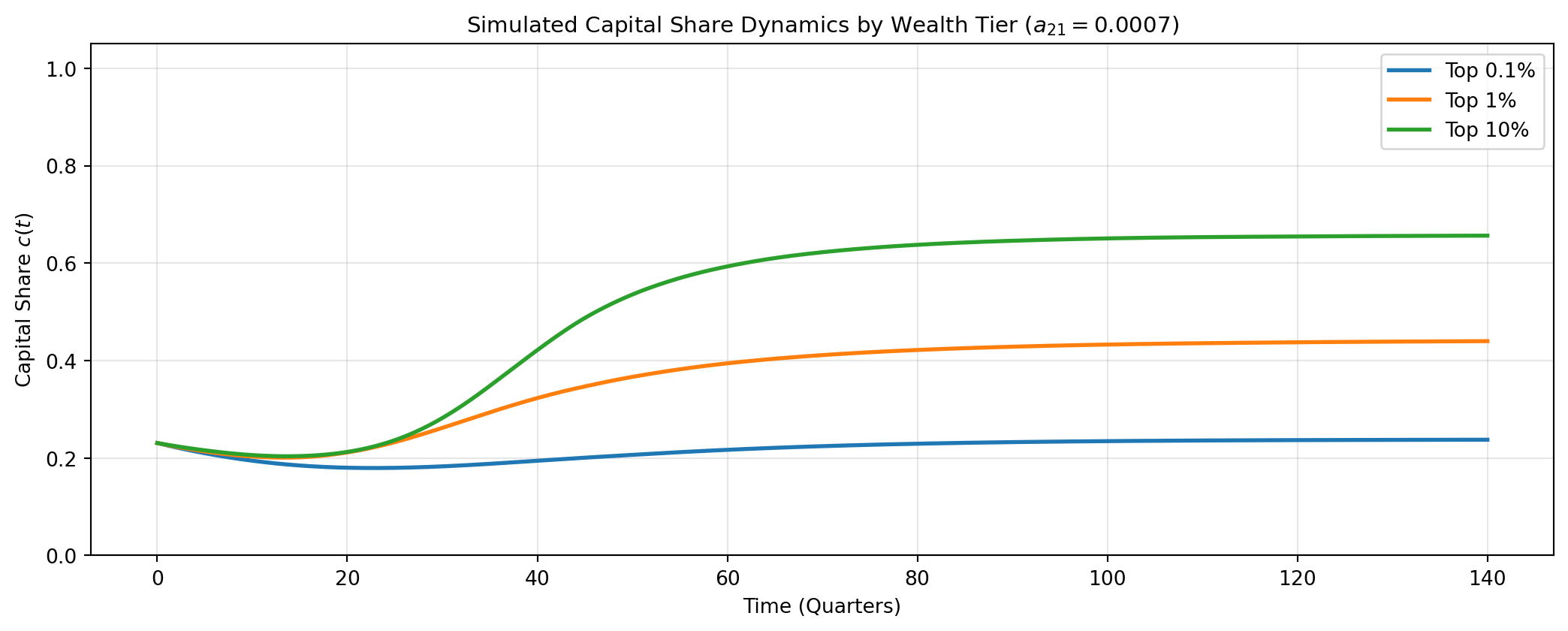
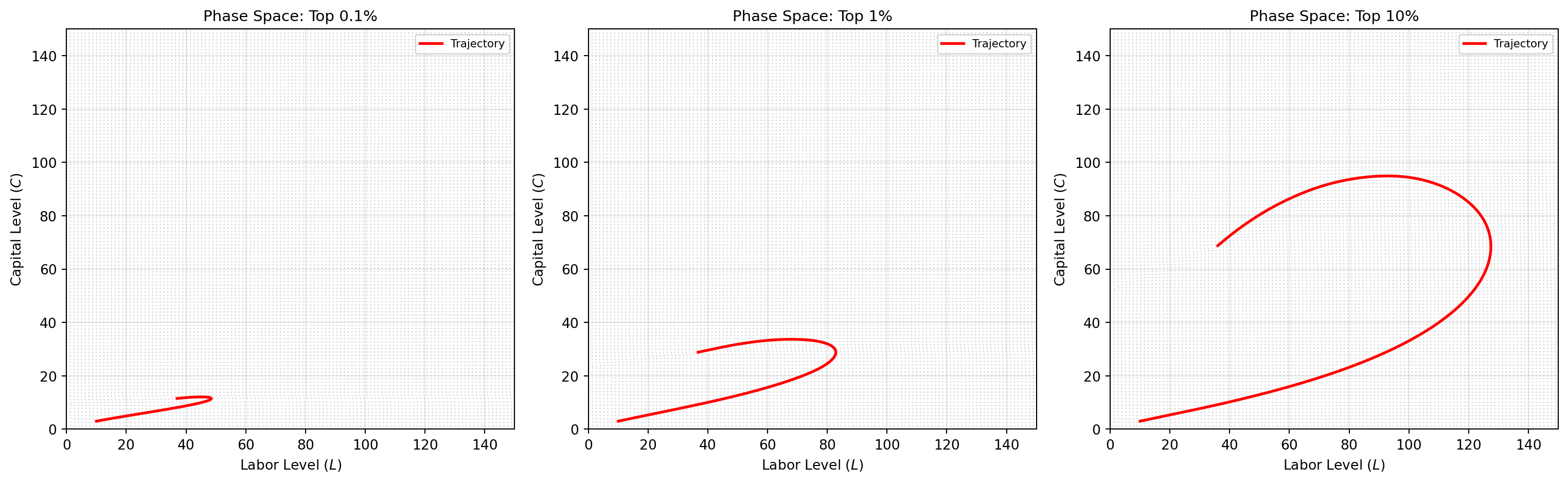
We numerically integrate the system using median parameters for each wealth tier under calibrated labor-driven capital accumulation (\(a_{21} = 0.0007\)).

def simulate_system(params_dict, L0=10.0, C0=3.0, t_span=(0, 140), t_steps=2000):
    def system(t, y):
        L, C = y
        dL = params_dict["a11"] * L - params_dict["a12"] * L * C
        dC = 0.0007 * L * C + params_dict["a22"] * C - params_dict["a23"] * C - params_dict["a24"] * C**2
        return [dL, dC]

    t_eval = np.linspace(t_span[0], t_span[1], t_steps)
    sol = solve_ivp(system, t_span, [L0, C0], t_eval=t_eval)
    return sol.t, sol.y[0], sol.y[1]

t, L_01, C_01 = simulate_system(params_top_01)
_, L_1, C_1 = simulate_system(params_top_1)
_, L_10, C_10 = simulate_system(params_top_10)

c_01 = C_01 / (L_01 + C_01)
c_1 = C_1 / (L_1 + C_1)
c_10 = C_10 / (L_10 + C_10)

plt.figure(figsize=(11, 4.5))
plt.plot(t, c_01, label="Top 0.1%", lw=2)
plt.plot(t, c_1, label="Top 1%", lw=2)
plt.plot(t, c_10, label="Top 10%", lw=2)
plt.title("Simulated Capital Share Dynamics by Wealth Tier ($a_{21} = 0.0007$)", fontsize=11)
plt.xlabel("Time (Quarters)")
plt.ylabel("Capital Share $c(t)$")
plt.ylim(0, 1.05)
plt.grid(True, alpha=0.3)
plt.legend()
plt.tight_layout()
plt.show()

Figure 4: Simulated Time-Domain Capital Share Dynamics \(c(t)\) for Each Percentile Group Using Calibrated \(a_{21} = 0.0007\).

L_vals = np.linspace(0, 150, 120)
C_vals = np.linspace(0, 150, 120)
L_grid, C_grid = np.meshgrid(L_vals, C_vals)

fig, axes = plt.subplots(1, 3, figsize=(16, 5))
group_dict = {
    "Top 0.1%": params_top_01,
    "Top 1%": params_top_1,
    "Top 10%": params_top_10
}

for ax, (label, p) in zip(axes, group_dict.items()):
    dL = p["a11"] * L_grid - p["a12"] * L_grid * C_grid
    dC = 0.0007 * L_grid * C_grid + p["a22"] * C_grid - p["a23"] * C_grid - p["a24"] * C_grid**2
    mag = np.sqrt(dL**2 + dC**2) + 1e-8
    
    ax.quiver(L_grid, C_grid, dL/mag, dC/mag, angles='xy', color='gray', alpha=0.45)
    t_sim, L_tr, C_tr = simulate_system(p)
    ax.plot(L_tr, C_tr, 'r-', lw=2, label='Trajectory')
    ax.set_title(f"Phase Space: {label}", fontsize=11)
    ax.set_xlabel("Labor Level $(L)$")
    ax.set_ylabel("Capital Level $(C)$")
    ax.set_xlim(0, 150)
    ax.set_ylim(0, 150)
    ax.grid(True, alpha=0.3)
    ax.legend(fontsize=8)

plt.tight_layout()
plt.show()

Figure 5: Level-Based Phase Space with Vector Fields and Simulated Trajectories across Top 0.1%, Top 1%, and Top 10% Wealth Tiers.

4.2 The Decoupling Paradox: Severance vs. Minimal Coupling

A central question emerges: can capital sustain itself indefinitely if labor is fully excluded?

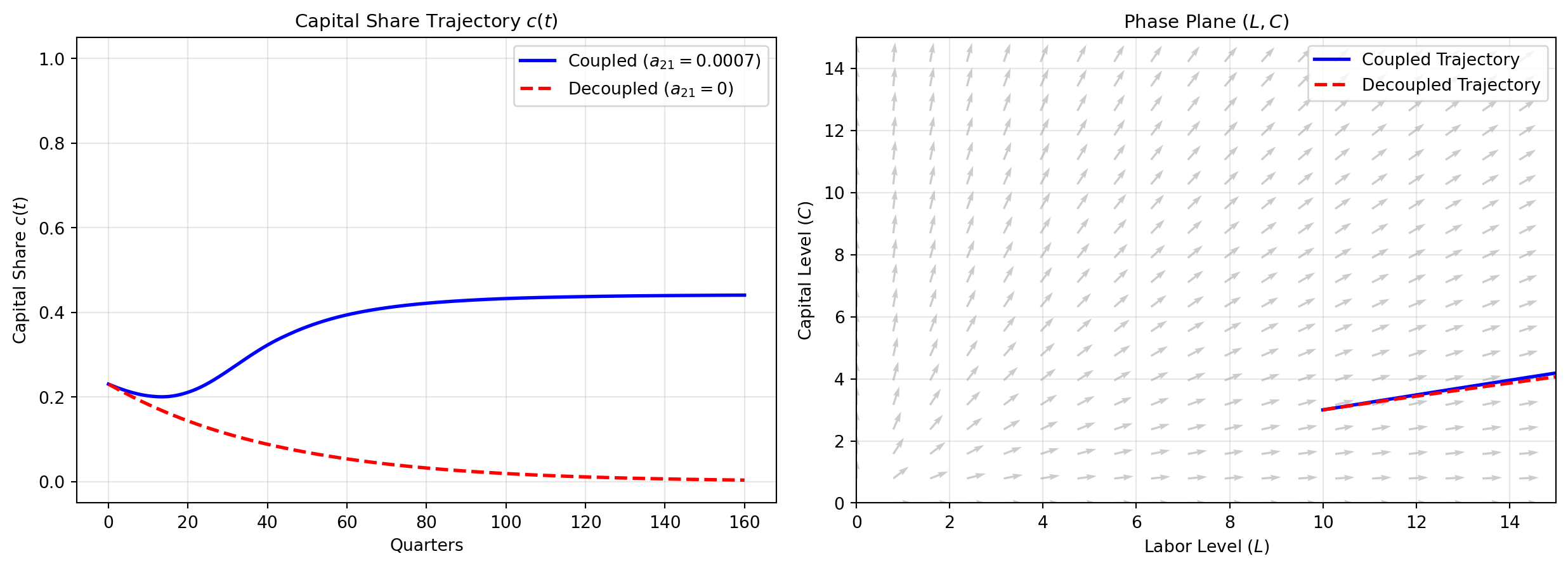
When \(a_{21} = 0\), the second differential equation reduces to autonomous capital growth tempered by depreciation and congestion: \(\dot{C} = (a_{22} - a_{23})C - a_{24}C^2\). While capital appears to enjoy self-sustaining autopoiesis in isolation, the disappearance of labor (\(L \to 0\)) dismantles the systemic demand and institutional substrate that underwrite asset valuation. In dynamic simulation, setting \(a_{21} = 0\) leads to a degenerate attractor: despite initial expansion, elite capital ultimately collapses under its own internal congestion and lack of systemic feedback.

Conversely, restoring an infinitesimal positive coupling—as small as \(a_{21} = 0.0007\)—fundamentally reorganizes the phase-space geometry, establishing an interior non-zero attractor where capital share stabilizes at realistic empirical ranges (0.30–0.70).

def simulate_paradox(a21_val, t_max=160):
    def ode_sys(t, y):
        L, C = y
        dL = params_top_1['a11'] * L - params_top_1['a12'] * L * C
        dC = a21_val * L * C + params_top_1['a22'] * C - params_top_1['a23'] * C - params_top_1['a24'] * (C**2)
        return [dL, dC]
    
    t_eval = np.linspace(0, t_max, 1000)
    sol = solve_ivp(ode_sys, (0, t_max), [10.0, 3.0], t_eval=t_eval)
    c_share = sol.y[1] / (sol.y[0] + sol.y[1])
    return sol.t, sol.y[0], sol.y[1], c_share

t, L_coupled, C_coupled, c_coupled = simulate_paradox(a21_val=0.0007)
_, L_severed, C_severed, c_severed = simulate_paradox(a21_val=0.0)

fig, (ax1, ax2) = plt.subplots(1, 2, figsize=(13, 4.8))

# Subplot 1: Share dynamics over time
ax1.plot(t, c_coupled, 'b-', lw=2, label=r'Coupled ($a_{21} = 0.0007$)')
ax1.plot(t, c_severed, 'r--', lw=2, label=r'Decoupled ($a_{21} = 0$)')
ax1.set_title("Capital Share Trajectory $c(t)$", fontsize=11)
ax1.set_xlabel("Quarters")
ax1.set_ylabel("Capital Share $c(t)$")
ax1.set_ylim(-0.05, 1.05)
ax1.grid(True, alpha=0.3)
ax1.legend()

# Subplot 2: Phase space vector field (Coupled)
L_grid_p, C_grid_p = np.meshgrid(np.linspace(0, 15, 20), np.linspace(0, 15, 20))
dL_p = params_top_1['a11'] * L_grid_p - params_top_1['a12'] * L_grid_p * C_grid_p
dC_p = 0.0007 * L_grid_p * C_grid_p + params_top_1['a22'] * C_grid_p - params_top_1['a23'] * C_grid_p - params_top_1['a24'] * C_grid_p**2
mag_p = np.sqrt(dL_p**2 + dC_p**2) + 1e-8

ax2.quiver(L_grid_p, C_grid_p, dL_p/mag_p, dC_p/mag_p, color='gray', alpha=0.4)
ax2.plot(L_coupled, C_coupled, 'b-', lw=2, label='Coupled Trajectory')
ax2.plot(L_severed, C_severed, 'r--', lw=2, label='Decoupled Trajectory')
ax2.set_title("Phase Plane $(L, C)$", fontsize=11)
ax2.set_xlabel("Labor Level $(L)$")
ax2.set_ylabel("Capital Level $(C)$")
ax2.set_xlim(0, 15)
ax2.set_ylim(0, 15)
ax2.grid(True, alpha=0.3)
ax2.legend()

plt.tight_layout()
plt.show()

Figure 6: The Decoupling Paradox: (A) Capital share simulation showing system stabilization with minimal coupling (\(a_{21}=0.0007\)) versus decay; (B) Phase space trajectories in \((L, C)\) plane exhibiting the boundary attractor.

5 Normative Implications

5.1 Equilibrium as Structural Exclusion

In classical welfare economics, equilibrium carries an implicit normative imprimatur—it represents Pareto optimality, market clearing, and the balance of competitive forces. Our dynamical results dismantle this equivalence. In a system characterized by non-conservative feedback and autopoietic capital accumulation, equilibrium is merely a constraint-compatible attractor determined by phase-space geometry.

When parameters cross the threshold where \(a_{22} > a_{23}\) and \(a_{21} \to 0\), the long-run stationary state is not an optimal clearing of factor markets, but the topological extinction of labor. To describe such a terminal state as an “equilibrium” confuses mathematical resting states with social viability.

5.2 Anticipatory Policy on System Curvature

Conventional economic policy relies almost exclusively on ex-post redistribution—allowing market mechanisms to generate primary inequality, followed by fiscal transfers (e.g., progressive income taxation, welfare subsidies).

However, dynamical systems theory reveals the fatal flaw of this approach: once a trajectory approaches an absorbing manifold (\(L \to 0\)), the basin of attraction becomes rigid. Compensatory transfers cannot revive an economically obsolete class whose structural transmission channels have been zeroed out.

Ethical economic design must operate as anticipatory geometry: intervening where phase-space curvature is flexible, before trajectories lock into degenerate attractors:

1. Re-anchoring Labor Transmission (\(a_{21}\)): Mandating structural equity participation, algorithmic co-ownership, and worker-held equity trusts that institutionally bind capital growth to labor welfare (\(a_{21} > 0\)).
2. Mitigating Elite Congestion (\(a_{24}\)): Introducing progressive wealth and asset-hoarding taxes targeting idle, speculative capital, thereby suppressing the destructive positional arms race among top percentiles.
3. Limiting Displacement Velocity (\(a_{12}\)): Instituting transition friction on rapid labor substitution to allow demographic and educational re-alignment.
4. Socializing Autopoietic Compounding (\(a_{22}\)): Ensuring sovereign, public ownership stakes in core AI infrastructure and general-purpose foundation models, preventing autopoietic compounding from remaining an exclusive elite monopoly.

6 Conclusion

The survival of economic systems under advanced automation is governed neither by moral desert nor static efficiency, but by the topological curvature of structural feedback. Capital self-replication without labor anchoring is inherently self-terminating. Preserving human agency in the AX era requires actively redesigning the phase space—transforming capital accumulation from an exclusionary closed loop into an endogenously coupled, stable architecture.

References

Acemoglu, Daron, and Pascual Restrepo. 2018. “The Race Between Man and Machine: Implications of Technology for Growth, Factor Shares, and Employment.” American Economic Review 108 (6): 1488–542.

Andrew Berg, Edward F. Buffie, and Luis-Felipe Zanna. 2018. “Should We Fear the Robot Revolution? (The Correct Answer Is Yes).” IMF Working Paper, no. 18/116.

Flaschel, Peter. 2009. The Macrodynamics of Capitalism: Elements for a Synthesis of Marx, Keynes and Schumpeter. Springer.

Goodwin, Richard M. 1967. A Growth Cycle. 54–58.

Lotka, Alfred J. 1925. Elements of Physical Biology. Williams; Wilkins Company.

Marx, Karl. 1867. Das Kapital: Kritik Der Politischen Ökonomie. Verlag von Otto Meisner.

Piketty, Thomas. 2014. Capital in the Twenty-First Century. Harvard University Press.

Seth Benzell, Guillermo LaGarda, Laurence Kotlikoff, and Jeffrey Sachs. 2015. “Robots Are Us: Some Economics of Human Replacement.” NBER Working Paper, no. 20941.

Susskind, Daniel. 2020. A World Without Work: Technology, Automation, and How We Should Respond. Metropolitan Books.

Volterra, Vito. 1926. “Fluctuations in the Abundance of a Species Considered Mathematically.” Nature 118: 558–60.