Regression Models

From Data Generating Processes to Geometries of Estimation

데이터 생성 과정(DGP) 관점에서 빈도주의 OLS와 베이지안 회귀(MCMC·깁스 샘플링), 칼만 필터 및 시변 계수(TVP) 모델의 수리통계적 기하학을 정합적으로 통합 비교한다.

Author

gitSAM

Published

September 15, 2026

A statistical regression model is a mathematical framework designed to separate signal from noise within observable data and to characterize conditional dependence structures between variables. For the problem of modeling the relationship between a scalar dependent variable \(y \in \mathbb{R}\) and a scalar independent variable \(x \in \mathbb{R}\), the rigorous point of departure is not algebraic line-fitting, but a probabilistic formulation of the Data Generating Process (DGP).

Depending on the underlying philosophical perspective, regression modeling bifurcates into two paradigms regarding foundational premises, the ontological status of parameters, and the distributional interpretation of estimators.

1 Frequentist Perspective: Fixed Parameters and Limiting Laws of Sampling Distributions

In the frequentist paradigm, the true parameter vector \(\beta = [\beta_0, \beta_1]^T\) is an unknown but fixed constant, analogous to a physical constant. Observed data variability reflects random sampling error arising from uncontrollable data generation and collection mechanisms, rather than parameter instability.

\[y_i = X_i^T \beta + \epsilon_i, \quad X_i = [1, x_i]^T, \quad i = 1, \dots, N\]

1.1 Assumptions of White Noise and Gaussian Isotropy

Modeling the error vector \(\epsilon = [\epsilon_1, \dots, \epsilon_N]^T\) as Gaussian white noise, \(\epsilon \sim \mathcal{N}(0, \sigma^2 I_N)\), stems from geometric and physical necessity rather than mere computational convenience.

To mathematically express the complete absence of prior directional bias in the error space \(\mathbb{R}^N\), the joint probability density function of the error vector must exhibit rotational symmetry—isotropy—remaining invariant under orthogonal transformations (rotations and reflections).

Let \(p(\epsilon)\) denote the joint probability density function of the error vector \(\epsilon\). Rotational invariance under any orthogonal matrix \(U\) (\(U^T U = I_N\)) implies \(p(\epsilon) = p(U\epsilon)\). This requires that \(p(\epsilon)\) depend solely on the squared Euclidean norm \(\Vert\epsilon\Vert^2 = \sum_{i=1}^N \epsilon_i^2\), expressed as a composite function \(g: \mathbb{R}_{\ge 0} \to \mathbb{R}\):

\[p(\epsilon) = g\left(\Vert{}\epsilon\Vert{}^2\right) = g\left(\sum_{i=1}^N \epsilon_i^2\right)\]

Combining this with the assumption of mutual independence among individual errors \(\epsilon_i\), we write \(p(\epsilon) = \prod_{i=1}^N p_i(\epsilon_i)\), where \(p_i(\epsilon_i)\) is the marginal density of the \(i\)-th error component. Taking the natural logarithm transforms the product into a sum:

\[\sum_{i=1}^N \ln p_i(\epsilon_i) = \ln g\left(\sum_{i=1}^N \epsilon_i^2\right)\]

Differentiating both sides with respect to any component \(\epsilon_j\) yields:

\[\frac{p_j'(\epsilon_j)}{\epsilon_j p_j(\epsilon_j)} = 2 \frac{g'\left(\sum_{i=1}^N \epsilon_i^2\right)}{g\left(\sum_{i=1}^N \epsilon_i^2\right)}\]

The left-hand side depends solely on \(\epsilon_j\), while the right-hand side depends on the total sum of squares \(\sum \epsilon_i^2\). Consequently, both expressions must equal an invariant constant across all components \(\epsilon_j\). If this constant were non-negative, the probability density function would diverge across the real line, violating the normalizability condition \(\int_{-\infty}^\infty p_j(\epsilon_j) d\epsilon_j = 1\). The constant must therefore be negative, \(-2c\) (\(c > 0\)), leading to \(\frac{p_j'(\epsilon_j)}{p_j(\epsilon_j)} = -2c \epsilon_j\). Integrating this differential equation uniquely yields the Gaussian density \(p_j(\epsilon_j) \propto \exp(-c \epsilon_j^2)\). The derivation of the normal distribution from rotational invariance (isotropy) and mutual component independence is known as the Maxwell-Herschel Theorem¹.

Information theory reaches the same conclusion. Among all continuous probability distributions with mean zero and fixed variance \(\sigma^2\), the Gaussian distribution uniquely maximizes differential entropy, \(H(p) = -\int p(\epsilon) \ln p(\epsilon) d\epsilon\). According to the Principle of Maximum Entropy, maximizing entropy represents the most conservative modeling choice, introducing the least subjective bias or unverified information beyond the specified moment constraints.

1.2 Estimator Distribution Interpretation via LLN and CLT

Under the frequentist framework, the Ordinary Least Squares (OLS) estimator \(\hat{\beta}\) is a function of the random sample \(Y\), making it a random variable itself:

\[\hat{\beta} = (X^T X)^{-1} X^T Y = \beta + \left(\frac{1}{N} X^T X\right)^{-1} \left(\frac{1}{N} X^T \epsilon\right)\]

The asymptotic validity and sampling properties of the estimator are established under the hypothetical repeated sampling of the data-generating process via limit theorems.

First, the Law of Large Numbers (LLN) establishes consistency. Under the independent and identically distributed (i.i.d.) assumption and finite moment conditions, sample moments converge in probability to population moments:

\[\frac{1}{N} X^T X \xrightarrow{P} \mathbb{E}[X_i X_i^T] = \Sigma_{XX}\]

\[\frac{1}{N} X^T \epsilon \xrightarrow{P} \mathbb{E}[X_i \epsilon_i] = 0\]

By Slutsky’s Theorem, asymptotic consistency follows:

\[\hat{\beta} \xrightarrow{P} \beta\]

Second, the Central Limit Theorem (CLT) establishes asymptotic normality even when the finite-sample error terms \(\epsilon_i\) deviate from exact normality. Under the Lindeberg-Lévy CLT:

\[\frac{1}{\sqrt{N}} X^T \epsilon \xrightarrow{d} \mathcal{N}(0, \sigma^2 \Sigma_{XX})\]

The asymptotic distribution of the standardized estimator is:

\[\sqrt{N}(\hat{\beta} - \beta) \xrightarrow{d} \mathcal{N}\left(0, \sigma^2 \Sigma_{XX}^{-1}\right)\]

A frequentist \(95\%\) confidence interval does not denote a \(95\%\) probability that the true parameter \(\beta\) lies within the specific realized interval. Instead, it represents frequentist coverage probability: across infinite hypothetical replications of the sampling and estimation procedure, \(95\%\) of the constructed intervals contain the fixed parameter \(\beta\).

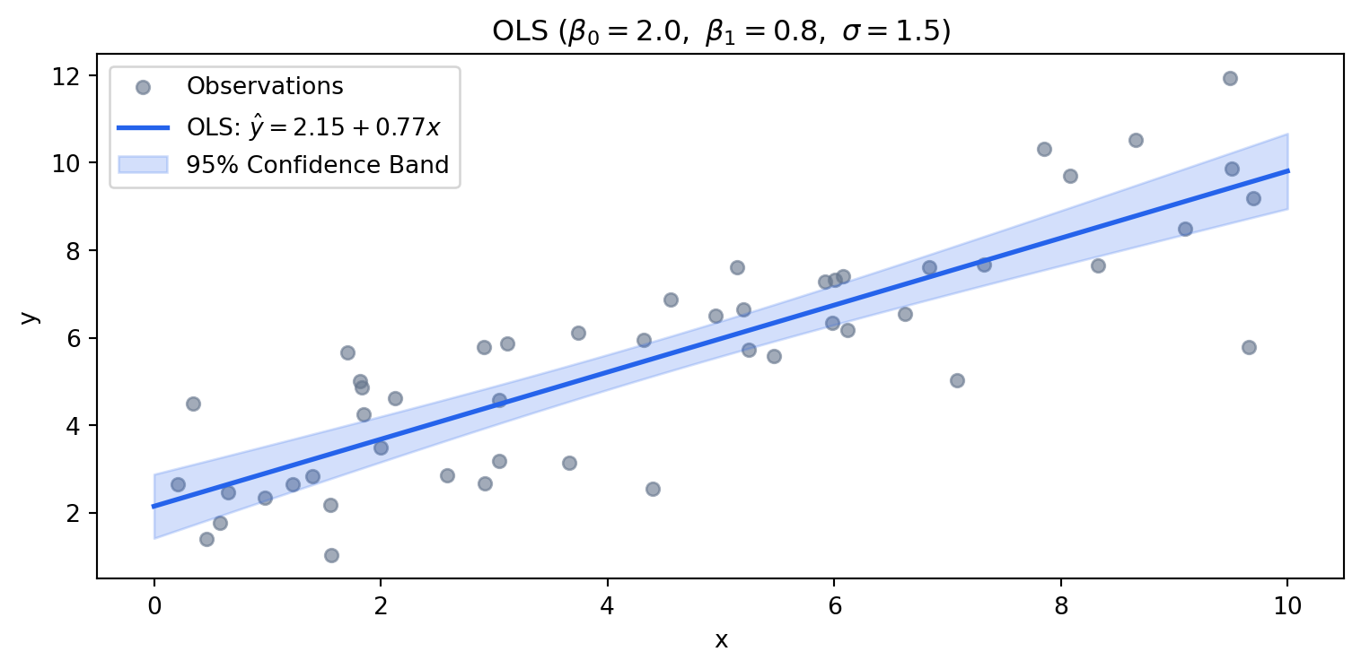
1.3 Example: OLS Estimation and Confidence Band Visualization

Samples are simulated from a known DGP, followed by computing closed-form OLS estimates and plotting the \(95\%\) confidence band.

Code

import numpy as np
import matplotlib.pyplot as plt
from scipy import stats

np.random.seed(42)

# ── DGP Setup ──
N = 50
beta_true = np.array([2.0, 0.8])   # [intercept, slope]
sigma = 1.5

x = np.random.uniform(0, 10, N)
X = np.column_stack([np.ones(N), x])
epsilon = np.random.normal(0, sigma, N)
y = X @ beta_true + epsilon

# ── OLS Estimation ──
beta_hat = np.linalg.inv(X.T @ X) @ X.T @ y
residuals = y - X @ beta_hat
sigma_hat_sq = np.sum(residuals**2) / (N - 2)
cov_beta = sigma_hat_sq * np.linalg.inv(X.T @ X)

# ── 95% Confidence Band ──
t_crit = stats.t.ppf(0.975, df=N - 2)
x_grid = np.linspace(0, 10, 200)
X_grid = np.column_stack([np.ones_like(x_grid), x_grid])
y_pred = X_grid @ beta_hat
se_mean = np.sqrt(np.diag(X_grid @ cov_beta @ X_grid.T))

fig, ax = plt.subplots(figsize=(8, 4))
ax.scatter(x, y, alpha=0.6, color="#64748b", s=30, label="Observations")
ax.plot(x_grid, y_pred, color="#2563eb", lw=2,
        label=rf"OLS: $\hat{{y}} = {beta_hat[0]:.2f} + {beta_hat[1]:.2f}x$")
ax.fill_between(x_grid,
                y_pred - t_crit * se_mean,
                y_pred + t_crit * se_mean,
                alpha=0.2, color="#2563eb", label="95% Confidence Band")
ax.set_xlabel("x")
ax.set_ylabel("y")
ax.set_title(rf"OLS ($\beta_0={beta_true[0]},\ \beta_1={beta_true[1]},\ \sigma={sigma}$)")
ax.legend()
plt.tight_layout()
plt.show()

print(f"True params  : beta_0 = {beta_true[0]:.3f}, beta_1 = {beta_true[1]:.3f}")
print(f"OLS estimates: beta_0 = {beta_hat[0]:.3f}, beta_1 = {beta_hat[1]:.3f}")
print(f"Estimated var: sigma^2 = {sigma_hat_sq:.3f}")

Figure 1: OLS Estimation with 95% Confidence Band

True params  : beta_0 = 2.000, beta_1 = 0.800
OLS estimates: beta_0 = 2.145, beta_1 = 0.766
Estimated var: sigma^2 = 1.929

2 Bayesian Perspective: Parameter Stochasticity and Conditional Joint Distributions

In the Bayesian framework, the parameter vector \(\beta\) is not treated as a fixed constant, but as a random variable quantifying the observer’s epistemic state and uncertainty.

2.1 Decomposition of the Conditional Joint Distribution \(p(X, Y \vert{} \beta)\) and Likelihood

In regression analysis, the primary object of inquiry is the relationship between the set of covariates \(X\) and targets \(Y\). Given parameter vector \(\beta\), the joint distribution of the data decomposes by the chain rule of probability:

\[p(X, Y \vert{} \beta) = p(Y \vert{} X, \beta) p(X \vert{} \beta)\]

Standard regression models impose an exogeneity assumption, positing that the marginal data-generating process of \(X\) contains no functional dependence on \(\beta\). Hence, \(p(X \vert{} \beta) = p(X)\), giving:

\[p(X, Y \vert{} \beta) = p(Y \vert{} X, \beta) p(X)\]

For inferring \(\beta\), the marginal density \(p(X)\) functions as an uninformative normalizing constant. The informative core reduces to the conditional likelihood of the response vector \(Y\) given inputs \(X\) and parameters \(\beta\):

\[p(Y \vert{} X, \beta) = \prod_{i=1}^N p(y_i \vert{} X_i, \beta) = (2\pi\sigma^2)^{-N/2} \exp\left(-\frac{1}{2\sigma^2} (Y - X\beta)^T (Y - X\beta)\right)\]

Specifying a prior distribution \(p(\beta)\) establishes the joint model over parameters and observed targets conditional on design inputs:

\[p(\beta, Y \vert{} X) = p(Y \vert{} X, \beta) p(\beta)\]

The posterior distribution is normalized by the marginal likelihood (evidence):

\[p(\beta \vert{} Y, X) = \frac{p(Y \vert{} X, \beta) p(\beta)}{\int p(Y \vert{} X, \beta) p(\beta) d\beta}\]

Under a conjugate Gaussian prior \(\beta \sim \mathcal{N}(\mu_0, \Sigma_0)\), completing the square inside the exponential combines the data precision (\(\frac{1}{\sigma^2} X^T X\)) and prior precision (\(\Sigma_0^{-1}\)), yielding a Gaussian posterior \(\mathcal{N}(\mu_N, \Sigma_N)\):

\[\Sigma_N = \left(\Sigma_0^{-1} + \frac{1}{\sigma^2} X^T X\right)^{-1}, \quad \mu_N = \Sigma_N \left(\Sigma_0^{-1} \mu_0 + \frac{1}{\sigma^2} X^T Y\right)\]

In the limit of an uninformative prior with precision approaching zero (\(\Sigma_0^{-1} \to 0\)), the posterior mean \(\mu_N\) coincides with the OLS estimator \(\hat{\beta}\). As sample size grows, the likelihood dominates the prior, leading frequentist and Bayesian inferences to asymptotically coincide.

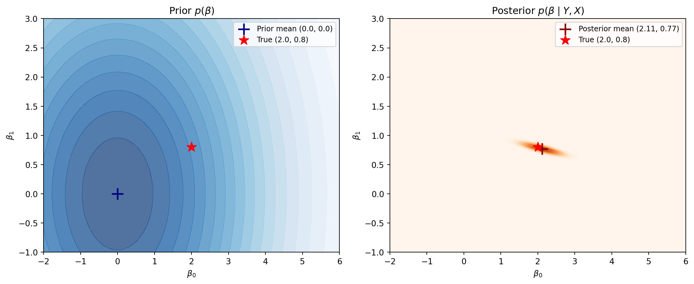
2.2 Example: Prior-to-Posterior Update under Conjugate Normal Prior

Using the simulated sample, the update from a weakly informative prior (\(\Sigma_0 = 10I\)) to the posterior distribution is illustrated via contour density plots.

Code

from scipy.stats import multivariate_normal

# ── Prior Setup ──
mu_0 = np.array([0.0, 0.0])
Sigma_0 = np.diag([10.0, 10.0])

# ── Conjugate Posterior Computation (known sigma^2) ──
sigma_sq = sigma**2
prec_prior = np.linalg.inv(Sigma_0)
prec_data  = (1 / sigma_sq) * X.T @ X

Sigma_N = np.linalg.inv(prec_prior + prec_data)
mu_N    = Sigma_N @ (prec_prior @ mu_0 + (1 / sigma_sq) * X.T @ y)

# ── Contour Visualization ──
b0_range = np.linspace(-2, 6, 200)
b1_range = np.linspace(-1, 3, 200)
B0, B1 = np.meshgrid(b0_range, b1_range)
pos = np.dstack((B0, B1))

prior_pdf     = multivariate_normal(mu_0, Sigma_0).pdf(pos)
posterior_pdf  = multivariate_normal(mu_N, Sigma_N).pdf(pos)

fig, axes = plt.subplots(1, 2, figsize=(12, 5))

ax = axes[0]
ax.contourf(B0, B1, prior_pdf, levels=20, cmap="Blues", alpha=0.7)
ax.scatter(*mu_0, color="navy", marker="+", s=200, lw=2,
           label=f"Prior mean ({mu_0[0]}, {mu_0[1]})")
ax.scatter(*beta_true, color="red", marker="*", s=150,
           label=f"True ({beta_true[0]}, {beta_true[1]})")
ax.set_xlabel(r"$\beta_0$"); ax.set_ylabel(r"$\beta_1$")
ax.set_title(r"Prior $p(\beta)$"); ax.legend(fontsize=9)

ax = axes[1]
ax.contourf(B0, B1, posterior_pdf, levels=20, cmap="Oranges", alpha=0.7)
ax.scatter(*mu_N, color="darkred", marker="+", s=200, lw=2,
           label=f"Posterior mean ({mu_N[0]:.2f}, {mu_N[1]:.2f})")
ax.scatter(*beta_true, color="red", marker="*", s=150,
           label=f"True ({beta_true[0]}, {beta_true[1]})")
ax.set_xlabel(r"$\beta_0$"); ax.set_ylabel(r"$\beta_1$")
ax.set_title(r"Posterior $p(\beta \mid Y, X)$"); ax.legend(fontsize=9)

plt.tight_layout()
plt.show()

print(f"Prior mean  : {mu_0}")
print(f"Posterior mean: {mu_N.round(3)}")
print(f"OLS estimate  : {beta_hat.round(3)}")

Figure 2: Conjugate Normal Prior to Posterior Update

Prior mean  : [0. 0.]
Posterior mean: [2.114 0.771]
OLS estimate  : [2.145 0.766]

2.3 High-Dimensional Inference: MCMC and Stationarity

When the noise variance \(\sigma^2\) is also treated as an unknown parameter, or when models incorporate hierarchical structures or non-linearities, analytically computing the marginal likelihood integral (evidence) becomes intractable. Markov Chain Monte Carlo (MCMC) methods approximate the intractable posterior distribution through sampling rather than direct integration.

The foundational principle of MCMC lies in designing an ergodic Markov chain that has the target posterior \(p(\theta \vert{} Y, X)\) as its unique stationary distribution. Provided the transition kernel satisfies the detailed balance condition, samples generated by the chain converge in distribution to the target posterior after a sufficient burn-in period, irrespective of initial values.

2.3.1 1. Gibbs Sampling

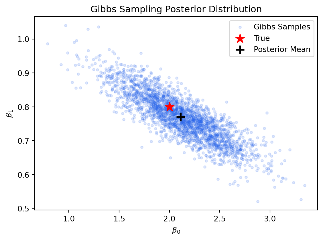
Gibbs sampling updates each component of the parameter vector \(\theta = (\beta, \sigma^2)\) iteratively by sampling directly from its full conditional posterior distribution given current values of all other parameters:

\[\beta^{(s+1)} \sim p(\beta \vert{} \sigma^{2(s)}, Y, X)\]

\[\sigma^{2(s+1)} \sim p(\sigma^2 \vert{} \beta^{(s+1)}, Y, X)\]

Under conditionally conjugate priors (such as Gaussian for regression coefficients and Inverse-Gamma for error variance), the full conditionals adopt closed-form analytical distributions, allowing direct draws without proposal rejections.

Code

# Gibbs sampler using full conditional posterior distributions
# beta | sigma^2, Y, X ~ Normal
# sigma^2 | beta, Y, X ~ Inverse-Gamma

n_samples = 3000
burn_in = 500

beta_samples_gibbs = np.zeros((n_samples, 2))
sigma2_samples_gibbs = np.zeros(n_samples)

# Initial values
beta_curr = np.array([0.0, 0.0])
sigma2_curr = 1.0

# Inverse-Gamma prior parameters (uninformative)
a_0, b_0 = 1.0, 1.0

XtX = X.T @ X
Xty = X.T @ y

for s in range(n_samples):
    # 1. Update beta (full conditional: multivariate normal)
    V_n = np.linalg.inv(prec_prior + (1.0 / sigma2_curr) * XtX)
    m_n = V_n @ (prec_prior @ mu_0 + (1.0 / sigma2_curr) * Xty)
    beta_curr = np.random.multivariate_normal(m_n, V_n)
    
    # 2. Update sigma^2 (full conditional: inverse-gamma)
    resid = y - X @ beta_curr
    a_n = a_0 + N / 2.0
    b_n = b_0 + 0.5 * np.sum(resid**2)
    # Generate Inverse-Gamma draw via reciprocal of Gamma draw
    sigma2_curr = 1.0 / np.random.gamma(a_n, 1.0 / b_n)
    
    beta_samples_gibbs[s] = beta_curr
    sigma2_samples_gibbs[s] = sigma2_curr

# Post burn-in samples
beta_post_gibbs = beta_samples_gibbs[burn_in:]

fig, ax = plt.subplots(figsize=(6, 4.5))
ax.scatter(beta_post_gibbs[:, 0], beta_post_gibbs[:, 1],
           alpha=0.15, color="#2563eb", s=10, label="Gibbs Samples")
ax.scatter(*beta_true, color="red", marker="*", s=150, zorder=5, label="True")
ax.scatter(*beta_post_gibbs.mean(axis=0), color="black", marker="+",
           s=120, lw=2, zorder=5, label="Posterior Mean")
ax.set_xlabel(r"$\beta_0$")
ax.set_ylabel(r"$\beta_1$")
ax.set_title("Gibbs Sampling Posterior Distribution")
ax.legend()
plt.tight_layout()
plt.show()

print(f"Gibbs Mean beta: {beta_post_gibbs.mean(axis=0).round(3)}")
print(f"Gibbs Mean sigma^2: {sigma2_samples_gibbs[burn_in:].mean():.3f}")

Figure 3: Gibbs Sampling for Bayesian Linear Regression

Gibbs Mean beta: [2.112 0.77 ]
Gibbs Mean sigma^2: 1.979

2.3.2 2. Metropolis-Hastings (MH)

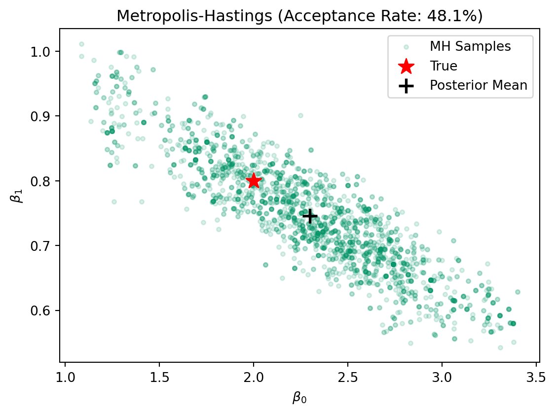
When full conditional distributions lack standard closed forms due to non-conjugacy or non-linearities, Gibbs sampling is inapplicable. The Metropolis-Hastings algorithm generates candidate states \(\theta^*\) from an arbitrary proposal distribution \(q(\theta^* \vert{} \theta^{(s)})\) and accepts them with probability \(\alpha\):

\[\alpha(\theta^{(s)}, \theta^*) = \min\left(1, \frac{p(Y \vert{} \theta^*) p(\theta^*) q(\theta^{(s)} \vert{} \theta^*)}{p(Y \vert{} \theta^{(s)}) p(\theta^{(s)}) q(\theta^* \vert{} \theta^{(s)})}\right)\]

Because the intractable normalizing constant in the denominator cancels out in the ratio, evaluating only the unnormalized target density (likelihood \(\times\) prior) suffices to guarantee convergence to the stationary distribution. When using a symmetric proposal distribution (\(q(\theta^* \vert{} \theta^{(s)}) = q(\theta^{(s)} \vert{} \theta^*)\)), such as a random walk Gaussian proposal, the acceptance probability reduces to the simple posterior odds ratio.

Code

# Random-walk Metropolis-Hastings algorithm (estimating beta with fixed sigma=1.5)

def log_posterior(beta_cand, X, y, sigma):
    # Log-Prior: Normal(0, 10 I)
    log_prior = -0.5 * np.sum(beta_cand**2 / 10.0)
    # Log-Likelihood
    resid = y - X @ beta_cand
    log_lik = -0.5 * N * np.log(2 * np.pi * sigma**2) - 0.5 * np.sum(resid**2) / (sigma**2)
    return log_prior + log_lik

beta_samples_mh = np.zeros((n_samples, 2))
beta_curr = np.array([0.0, 0.0])
log_p_curr = log_posterior(beta_curr, X, y, sigma)

proposal_step = 0.08
n_accepted = 0

for s in range(n_samples):
    beta_prop = beta_curr + np.random.normal(0, proposal_step, size=2)
    log_p_prop = log_posterior(beta_prop, X, y, sigma)
    
    # Acceptance probability in log scale
    log_alpha = log_p_prop - log_p_curr
    if np.log(np.random.uniform(0, 1)) < log_alpha:
        beta_curr = beta_prop
        log_p_curr = log_p_prop
        n_accepted += 1
        
    beta_samples_mh[s] = beta_curr

beta_post_mh = beta_samples_mh[burn_in:]

fig, ax = plt.subplots(figsize=(6, 4.5))
ax.scatter(beta_post_mh[:, 0], beta_post_mh[:, 1],
           alpha=0.15, color="#059669", s=10, label="MH Samples")
ax.scatter(*beta_true, color="red", marker="*", s=150, zorder=5, label="True")
ax.scatter(*beta_post_mh.mean(axis=0), color="black", marker="+",
           s=120, lw=2, zorder=5, label="Posterior Mean")
ax.set_xlabel(r"$\beta_0$")
ax.set_ylabel(r"$\beta_1$")
ax.set_title(f"Metropolis-Hastings (Acceptance Rate: {n_accepted/n_samples:.1%})")
ax.legend()
plt.tight_layout()
plt.show()

print(f"MH Mean beta: {beta_post_mh.mean(axis=0).round(3)}")

Figure 4: Metropolis-Hastings Algorithm for Linear Regression

MH Mean beta: [2.297 0.746]

3 Time-Series Dynamic Regression: State-Space Models and the Markov Property

To accommodate structural changes where regression coefficients evolve over time \(t = 1, \dots, T\), the static model is extended into a dynamic linear State-Space Model (SSM).

3.1 Markov Property and Algebraic Conditions of the State Transition Matrix

The state vector \(\beta_t = [\beta_{0,t}, \beta_{1,t}]^T \in \mathbb{R}^m\) represents unobserved latent states. The state-space architecture is governed by the first-order Markov property: conditional on the entire past history \(\{\beta_0, \dots, \beta_{t-1}\}\), the probability distribution of the current state \(\beta_t\) depends solely on the immediate predecessor \(\beta_{t-1}\):

\[p(\beta_t \vert{} \beta_{0:t-1}) = p(\beta_t \vert{} \beta_{t-1})\]

A linear Gaussian state-space model is formulated via a state transition equation and an observation equation. Incorporating an optional control input vector \(u_t \in \mathbb{R}^l\), the system is written as:

State transition equation:

\[\beta_t = F_t \beta_{t-1} + B_t u_t + w_t, \quad w_t \sim \mathcal{N}(0, Q_t)\]

Observation equation:

\[y_t = H_t \beta_t + D_t u_t + v_t, \quad v_t \sim \mathcal{N}(0, R_t)\]

The structural components and algebraic properties of these matrices are defined as follows:

State Transition Matrix (\(F_t \in \mathbb{R}^{m \times m}\)): Dictates the autonomous internal dynamics of the latent state. In a time-invariant system (\(F_t = F\)), asymptotic stability requires that all eigenvalues of \(F\) lie strictly within the unit circle (\(\vert{}\lambda_i(F)\vert{} < 1\)). If eigenvalues lie on the unit circle (\(\vert{}\lambda_i\vert{} = 1\)), the system is marginally stable, and presence of process noise \(w_t\) causes state variance to diverge over time. In random-walk specifications (\(F = I\)), the state follows a non-stationary integrated process.
Control Input Matrix (\(B_t \in \mathbb{R}^{m \times l}\)): Projects external control inputs \(u_t\) into state transitions.
Observation Matrix (\(H_t \in \mathbb{R}^{p \times m}\)): Maps the latent state into the observation space. For scalar univariate regression (\(p=1\)), \(H_t = [1, x_t]\).
Direct Transmission Matrix (\(D_t \in \mathbb{R}^{p \times l}\)): Captures direct feedthrough from control inputs to observations, typically zero in standard regression settings.
Noise Covariance Matrices (\(Q_t \in \mathbb{R}^{m \times m}, R_t \in \mathbb{R}^{p \times p}\)): Symmetric positive semi-definite matrices governing process disturbance and measurement noise, respectively.

4 Bayesian Filtering vs. Smoothing Mechanisms

In state-space formulations, the objective of Bayesian inference depends on the temporal horizon of the conditioning information set. Let \(Y_{1:t} = \{y_1, \dots, y_t\}\) denote observations available up to time \(t\).

4.1 Bayesian Filtering (Forward Recursion, Real-Time Tracking)

Filtering computes the conditional posterior distribution of the current state based on data observed up to the current time step \(t\):

\[p(\beta_t \vert{} Y_{1:t})\]

The Kalman Filter evaluates this distribution analytically for linear Gaussian models:

State Prediction: Propagates the prior state forward through the transition dynamics (Chapman-Kolmogorov equation):

\[\beta_{t\vert{}t-1} = F_t \beta_{t-1\vert{}t-1} + B_t u_t\]

\[P_{t\vert{}t-1} = F_t P_{t-1\vert{}t-1} F_t^T + Q_t\]

Measurement Update: Corrects the predicted mean and covariance using the measurement innovation (\(y_t - H_t \beta_{t\vert{}t-1}\)) weighted by the Kalman Gain \(K_t\):

\[K_t = P_{t\vert{}t-1} H_t^T (H_t P_{t\vert{}t-1} H_t^T + R_t)^{-1}\]

\[\beta_{t\vert{}t} = \beta_{t\vert{}t-1} + K_t (y_t - H_t \beta_{t\vert{}t-1})\]

\[P_{t\vert{}t} = (I - K_t H_t) P_{t\vert{}t-1}\]

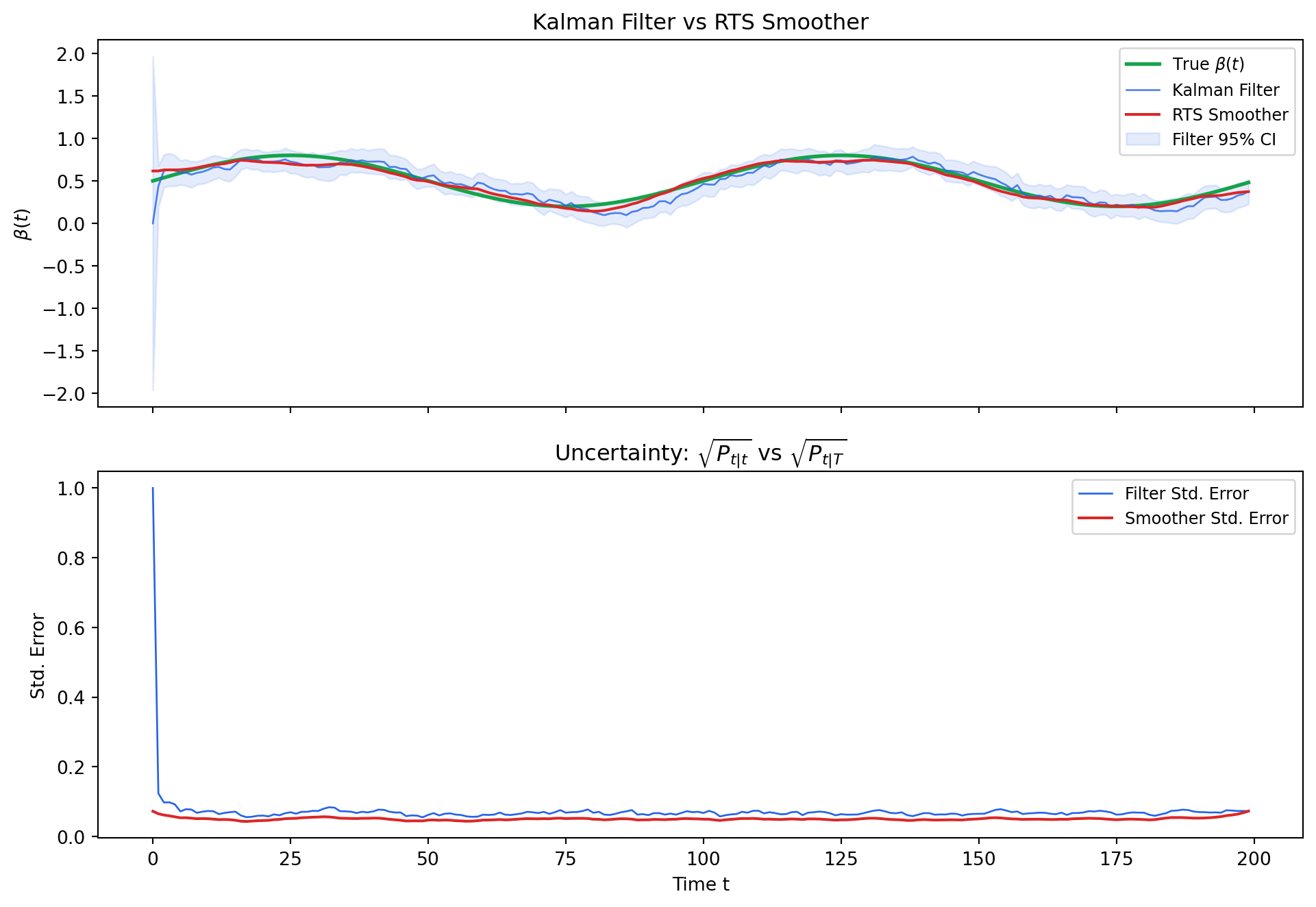
Because the filtered estimate \(\beta_{t\vert{}t}\) is strictly causal—relying only on past and contemporaneous information—it cannot anticipate future shocks. Under noisy observations, filtered trajectories inevitably display phase lag and high-frequency noise.

4.2 Bayesian Smoothing (Backward Recursion, Full-Trajectory Reconstruction)

Smoothing reconstructs the state distribution at an arbitrary past point \(t\) (\(t < T\)) after collecting the entire observation sequence \(Y_{1:T}\) up to time \(T\):

\[p(\beta_t \vert{} Y_{1:T})\]

The Rauch-Tung-Striebel (RTS) smoother retains the forward filter estimates and executes backward recursions from \(t = T-1, T-2, \dots, 1\):

\[J_t = P_{t\vert{}t} F_{t+1}^T P_{t+1\vert{}t}^{-1}\]

\[\beta_{t\vert{}T} = \beta_{t\vert{}t} + J_t (\beta_{t+1\vert{}T} - \beta_{t+1\vert{}t})\]

\[P_{t\vert{}T} = P_{t\vert{}t} + J_t (P_{t+1\vert{}T} - P_{t+1\vert{}t}) J_t^T\]

Here, \(J_t\) denotes the smoother gain matrix. The innovation term \(\beta_{t+1\vert{}T} - \beta_{t+1\vert{}t}\) reflects the revision between the smoothed trajectory at \(t+1\) and the one-step forward forecast. This adjustment propagates backward via \(J_t\) into state \(\beta_{t\vert{}t}\).

The smoothed covariance is guaranteed to be no greater than the filtered covariance in the matrix Loewner order, \(P_{t\vert{}T} \preceq P_{t\vert{}t}\). Because \(P_{t+1\vert{}T} \preceq P_{t+1\vert{}t}\), the difference \(P_{t+1\vert{}T} - P_{t+1\vert{}t}\) is negative semi-definite. Congruence transformations preserve semi-definiteness: \(J_t(P_{t+1\vert{}T} - P_{t+1\vert{}t})J_t^T \preceq 0\). Thus:

\[P_{t\vert{}T} = P_{t\vert{}t} + \underbrace{J_t (P_{t+1\vert{}T} - P_{t+1\vert{}t}) J_t^T}_{\preceq\, 0} \preceq P_{t\vert{}t}\]

Conditioning on future data retroactively narrows uncertainty, eliminating phase lag and delivering the minimum-variance trajectory across the full sample.

4.3 Example: Kalman Filter vs. RTS Smoother Comparison

The script below generates observations from a time-varying coefficient DGP, \(\beta(t) = 0.5 + 0.3\sin(2\pi t / 100)\), and estimates trajectories using both a Kalman filter and an RTS smoother under a random walk state specification. The lower panel validates that smoother variance remains strictly bounded by filter variance.

Code

np.random.seed(123)

T = 200
# Time-varying regression coefficient: beta(t) = 0.5 + 0.3 * sin(2*pi*t / 100)
t_idx = np.arange(T)
beta_true_t = 0.5 + 0.3 * np.sin(2 * np.pi * t_idx / 100)
x_t = np.random.normal(3, 1, T)
sigma_obs = 0.5
y_t = beta_true_t * x_t + np.random.normal(0, sigma_obs, T)

# State space: beta_t = beta_{t-1} + w_t,  y_t = x_t * beta_t + v_t
Q = 0.001          # Process noise variance
R = sigma_obs**2   # Measurement noise variance

# ── Kalman Filter (Forward) ──
beta_f = np.zeros(T)
P_f    = np.zeros(T)
beta_p = np.zeros(T)
P_p    = np.zeros(T)

beta_f[0], P_f[0] = 0.0, 1.0

for t in range(1, T):
    beta_p[t] = beta_f[t - 1]
    P_p[t]    = P_f[t - 1] + Q
    S         = x_t[t]**2 * P_p[t] + R
    K         = P_p[t] * x_t[t] / S
    beta_f[t] = beta_p[t] + K * (y_t[t] - x_t[t] * beta_p[t])
    P_f[t]    = (1 - K * x_t[t]) * P_p[t]

# ── RTS Smoother (Backward) ──
beta_s = beta_f.copy()
P_s    = P_f.copy()

for t in range(T - 2, -1, -1):
    J         = P_f[t] / P_p[t + 1]
    beta_s[t] = beta_f[t] + J * (beta_s[t + 1] - beta_p[t + 1])
    P_s[t]    = P_f[t] + J**2 * (P_s[t + 1] - P_p[t + 1])

# ── Visualization ──
fig, axes = plt.subplots(2, 1, figsize=(10, 7), sharex=True)

ax = axes[0]
ax.plot(t_idx, beta_true_t, color="#16a34a", lw=2, label=r"True $\beta(t)$")
ax.plot(t_idx, beta_f, color="#2563eb", lw=1, alpha=0.8, label="Kalman Filter")
ax.plot(t_idx, beta_s, color="#dc2626", lw=1.5, label="RTS Smoother")
ax.fill_between(t_idx,
                beta_f - 1.96 * np.sqrt(P_f),
                beta_f + 1.96 * np.sqrt(P_f),
                alpha=0.12, color="#2563eb", label="Filter 95% CI")
ax.set_ylabel(r"$\beta(t)$")
ax.set_title("Kalman Filter vs RTS Smoother")
ax.legend(fontsize=9, loc="upper right")

ax = axes[1]
ax.plot(t_idx, np.sqrt(P_f), color="#2563eb", lw=1, label="Filter Std. Error")
ax.plot(t_idx, np.sqrt(P_s), color="#dc2626", lw=1.5, label="Smoother Std. Error")
ax.set_xlabel("Time t")
ax.set_ylabel("Std. Error")
ax.set_title(r"Uncertainty: $\sqrt{P_{t|t}}$ vs $\sqrt{P_{t|T}}$")
ax.legend(fontsize=9)

plt.tight_layout()
plt.show()

Figure 5: Kalman Filter vs RTS Smoother for Time-Varying Regression

5 Cross-Sectional and Time-Series Comparative Summary

Dimension	Frequentist Approach	Bayesian Approach
Ontological Status of Parameter \(\beta\)	Unknown but fixed constant	Random variable formalizing uncertainty
Justification for Error Distribution	Rotational invariance (isotropy) & maximum entropy	Gaussian likelihood under absence of prior bias
Inference Framework	LLN (consistency) & CLT (asymptotic normality) under repeated sampling	Posterior updating based on conditional joint distribution
Computational Paradigm	Loss minimization and convex optimization (OLS, MLE)	Integral evaluation and simulation (MCMC, Gibbs, Metropolis-Hastings)
Dynamic Extension	Rolling window regressions, local polynomial least squares	Kalman filter (real-time tracking) & RTS smoother (full reconstruction)
Information Boundary	Fixed statistics on a single realized dataset	Causal tracking (\(Y_{1:t}\)) vs. acausal full reconstruction (\(Y_{1:T}\))

6 From Euclidean Geometry to Metric Deformations

The preceding sections formulated regression models under the foundational assumption that the data generating process (DGP) exhibits spherical Gaussian disturbances (\(\epsilon \sim \mathcal{N}(0, \sigma^2 I)\)) and spatial isotropy. Within this canonical setting, the Ordinary Least Squares (OLS) estimator arises naturally as an orthogonal projection onto the design column space, minimizing the standard Euclidean norm of the residual vector.

In empirical econometrics and observational data settings, however, heteroskedasticity and autocorrelation violate this isotropic residual geometry. Furthermore, when endogenous regressors or non-linear structural constraints arise, minimizing residual Euclidean norms ceases to yield consistent or efficient estimators, necessitating frameworks grounded in population moment conditions.

The following sections extend the geometric view of estimation from standard Euclidean projections (OLS) to metric-deformed residual spaces governed by positive definite kernels (GLS), and ultimately to the orthogonality of empirical moment conditions (GMM). In parallel, we explore the structural isomorphism between estimation theory—where informational precision deforms the loss geometry—and Einstein’s Field Equations in general relativity, where matter-energy distributions shape the Riemannian metric tensor of spacetime.

7 Linear to Curved Structures: Inner Product, Projection, and Positive Definite Kernels

7.1 OLS as Orthogonal Projection in Euclidean Space

OLS solves the following problem:

\[ \hat{\beta}_{OLS} = \arg\min_\beta \| y - X\beta \|_2^2 = (X^\top X)^{-1} X^\top y \]

This corresponds to projecting \(y\) orthogonally onto the column space of \(X\).
The residual \(\varepsilon = y - X\hat{\beta}\) satisfies:

\[ X^\top \varepsilon = 0 \]

7.1.1 Inner Product and Geometry

The \(L^2\) norm used in OLS is induced by the standard Euclidean inner product:

\[ \langle u, v \rangle = u^\top v \]

The distance function becomes:

\[ \| u \|_2 = \sqrt{u^\top u} \]

The set of parameter values yielding equal error defines a level set (isocurve):

\[ \{ \beta \mid \| y - X\beta \|_2^2 = c \} \Rightarrow \text{spheres in parameter space} \]

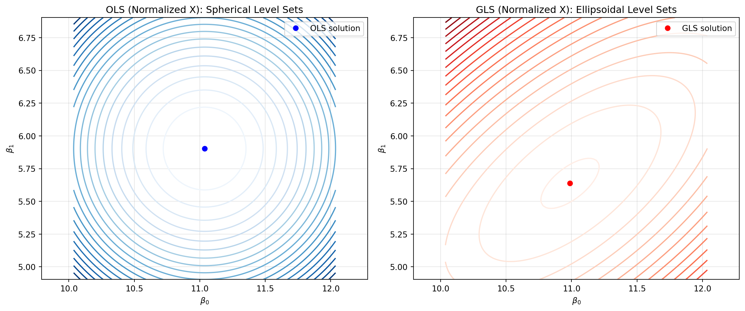
This reflects Pythagorean geometry — the isocurves are circles (in 2D), spheres (in 3D), or hyperspheres in higher dimensions when \(X^\top X = I\); otherwise, elliptical.
In this sense, OLS performs Euclidean projection onto a linear subspace using the standard inner product.

7.2 Generalized Least Squares (GLS)

GLS extends OLS by accounting for non-spherical error covariance structure:

\[ \hat{\beta}_{GLS} = \arg\min_\beta (y - X\beta)^\top \Sigma^{-1} (y - X\beta) \]

Here, \(\Sigma\) is the covariance matrix of the errors.
This defines a new inner product over the residual space:

\[ \langle u, v \rangle_\Sigma = u^\top \Sigma^{-1} v \]

The level sets:

\[ \{ \beta \mid (y - X\beta)^\top \Sigma^{-1} (y - X\beta) = c \} \Rightarrow \text{ellipsoids in parameter space} \]

This reflects how different directions in parameter space are penalized differently depending on the variance and correlation structure of the errors.

The ellipsoidal level sets visualized later correspond precisely to this GLS structure.

7.3 GMM as Orthogonality of Moment Conditions (Not Projection)

GMM generalizes the estimation framework by relying on moment conditions, not residuals:

\[ \hat{\theta}_{GMM} = \arg\min_\theta \left[ \bar{g}_n(\theta)^\top W \bar{g}_n(\theta) \right] \]

where:

\(\bar{g}_n(\theta) = \frac{1}{n} \sum_{i=1}^n g(Z_i, \theta)\) is the sample mean of moment functions
\(W\) is a positive definite weighting matrix, usually the inverse of the estimated variance of \(\bar{g}_n(\theta)\)

7.3.1 Clarifying the Inner Product

Although GMM also defines a quadratic form like GLS, it operates in a fundamentally different space:

In GLS: \(u, v\) are residual vectors
In GMM: \(u, v\) are moment function evaluations

Thus, while one can write:

\[ \langle g_i(\theta), g_j(\theta) \rangle_W = g_i(\theta)^\top W g_j(\theta) \]

it is important to emphasize:

GMM is not a projection-based method. It minimizes the violation of moment orthogonality conditions in expectation.

The isocurves:

\[ \{ \theta \mid \bar{g}_n(\theta)^\top W \bar{g}_n(\theta) = c \} \]

may also appear elliptical — but they are not projections, and should not be conflated with GLS geometrically.

7.3.2 Local Approximation and Connection to GLS

In some cases, GMM can be viewed as a local GLS approximation. If moment conditions are close to linear in \(\theta\), and \(g(Z_i, \theta) \approx A(Z_i)(\theta - \theta_0)\), then the GMM objective becomes:

\[ (\theta - \theta_0)^\top A^\top W A (\theta - \theta_0) \]

which resembles GLS — but only locally and approximately.

Therefore, the geometric intuition of ellipsoids applies more precisely to GLS. For GMM, it’s a useful visual aid — but structurally distinct.

7.4 Einstein Field Equations and GMM: Structural Analogy

Einstein’s Field Equations (EFE) in general relativity:

\[ G_{\mu\nu} = R_{\mu\nu} - \frac{1}{2} R g_{\mu\nu} = 8\pi T_{\mu\nu} \]

where:

\(T_{\mu\nu}\): Stress-energy tensor, representing energy and matter (matter-energy distribution)
\(G_{\mu\nu}\): Einstein tensor, encoding the curvature of spacetime (curvature)
- \(R_{\mu\nu}\): Ricci curvature tensor
- \(R\): Scalar curvature
- \(g_{\mu\nu}\): Metric tensor, defining the inner product in spacetime and governing geodesics

7.4.1 Analogy to Estimation Frameworks

Feature	OLS	GLS	GMM	EFE (Physics)
Space	Euclidean	Covariance-weighted	Moment function space	Curved spacetime
Inner product	\(I\)	\(\Sigma^{-1}\)	\(W\) (moment-weighted)	\(g_{\mu\nu}\) (metric)
Optimization	Projection	Weighted projection	Moment orthogonality	Energy-curvature balance
Level sets	Circles	Ellipses	Ellipsoid-like	Lightcones / geodesics

7.4.2 Lightcones and Degenerate Conics

In EFE, the metric tensor \(g_{\mu\nu}\) defines how distances and angles are measured — it is the analogue of a positive definite kernel in GMM. The field equations determine how the geometry (curvature) of spacetime reacts to matter and energy. In this sense, spacetime is optimized or shaped in response to external inputs, just as GMM shapes its estimation space based on the kernel \(W\) and moment functions.

The level sets in general relativity are often visualized as lightcones — the surface separating causal influence from spacelike separation. Geometrically, a lightcone can be interpreted as the degenerate case of a conic section, where the quadric form:

\[ Q(x) = x^\top g_{\mu\nu} x = 0 \]

results in a pair of intersecting lines: this represents all null (light-like) directions emanating from a point. These are the boundary cases between time-like and space-like intervals, analogous to the way ellipsoids in GMM collapse into degenerate forms under singular kernel matrices.

Thus, in both GMM and EFE, the shape and degeneracy of level sets encode deep information about the underlying structure — whether it is a statistical model or the geometry of spacetime.

7.5 Summary: Geometric Hierarchy of Estimation

OLS performs Euclidean projection in a space endowed with the standard inner product.
GLS generalizes this using a positive definite kernel over the residual space, yielding ellipsoidal level sets.
GMM further generalizes the concept by applying positive definite weighting over moment function space, not residuals.
Geometric analogies (spheres and ellipsoids) are structurally valid for OLS and GLS, and visually helpful — but must be used with care in GMM.
All three frameworks share a unifying theme: geometry induced by positive definite structure.

“OLS and GLS estimate by projection. GMM estimates by aligning empirical moments. Einstein’s theory bends space to match mass — estimation theory bends geometry to match data.”

7.6 Visuals & Empirical Demonstrations

7.6.1 OLS vs. GLS: Different Projections Under the Same Linear Model

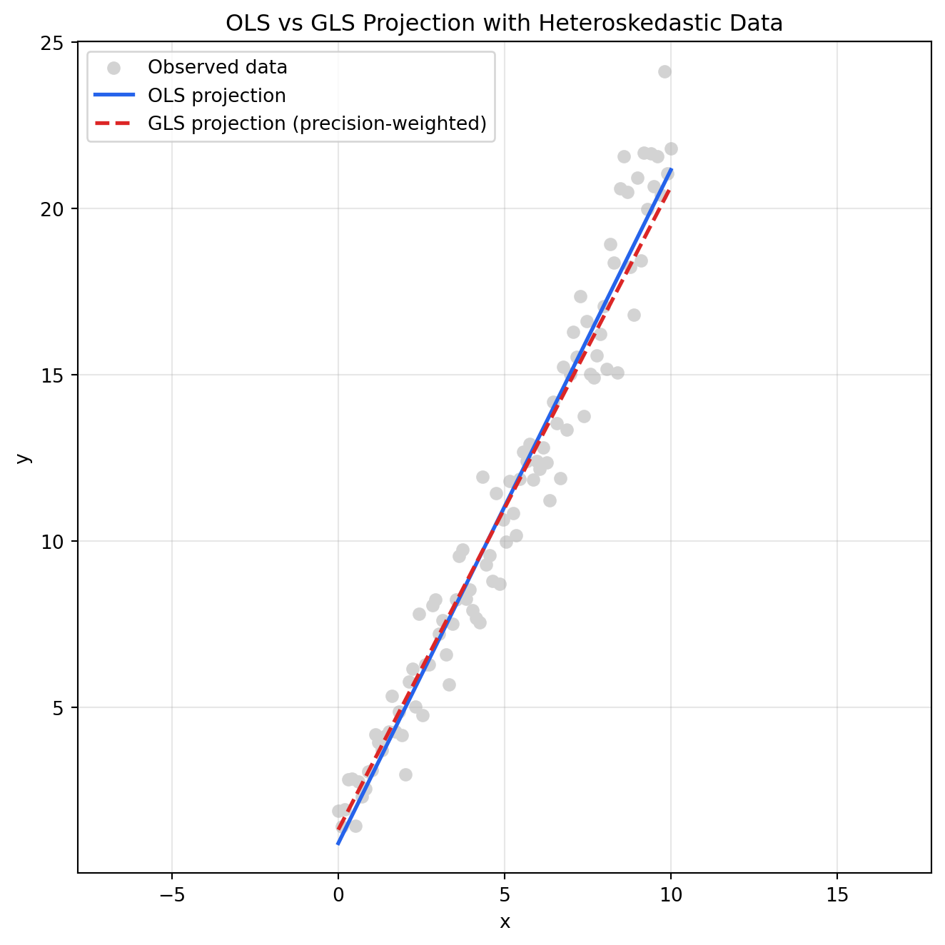
This section visualizes how OLS and GLS (with heteroskedastic weighting) yield different estimators even under the same linear model structure. The key distinction lies in how each method defines distance and importance via its respective inner product.

7.6.1.1 Simulation Setup

Data-generating process: \[ y = \beta_0 + \beta_1 x + \varepsilon \] where the noise term \(\varepsilon\) is heteroskedastic — its variance increases with \(x\).
That is, the reliability of observations decreases toward the right end of the domain.
OLS estimation:
- Minimizes the unweighted squared residuals: \[ \min_\beta \| y - X\beta \|_2^2 \]
- Assumes all observations are equally informative.
- The projection balances the residuals across the entire domain, including high-noise regions.
GLS estimation:
- Minimizes a precision-weighted residual norm: \[ \min_\beta (y - X\beta)^\top W (y - X\beta) \] where \(W\) is a positive definite diagonal matrix with weights inversely proportional to the noise variance.
- Observations with lower noise (on the left) are more heavily weighted.
- The resulting projection is skewed toward the low-variance region, yielding a steeper estimated slope.

7.6.1.2 Interpretation

Even though both methods fit a linear model, they differ fundamentally in the geometry of projection: - OLS projects onto the column space of \(X\) using the standard Euclidean inner product. - GLS projects in a space where the residuals are measured using a Mahalanobis-type norm, effectively reshaping the loss geometry.

This difference becomes visually striking when we compare their fitted lines on heteroskedastic data — OLS follows the average trend, while GLS emphasizes the cleaner data and suppresses the noisy part.

Code

import numpy as np
import matplotlib.pyplot as plt

# Simulate data with heteroskedastic noise (to favor GMM adjustment)
np.random.seed(0)
n = 100
x = np.linspace(0, 10, n)
X = np.vstack([np.ones(n), x]).T

# True model
beta_true_het = np.array([1, 2])
# Heteroskedastic noise: variance increases with x
noise_std = 0.5 + 1.5 * (x / x.max())  # ranges from 0.5 to 2.0
y_het = X @ beta_true_het + np.random.normal(0, noise_std)

# OLS estimation
beta_ols_het = np.linalg.inv(X.T @ X) @ X.T @ y_het
y_hat_ols_het = X @ beta_ols_het

# GLS/GMM weighting: inverse of variance (precision weighting)
W = np.diag(1 / noise_std**2)

# GLS estimation (optimal weighting under heteroskedasticity)
XTWX = X.T @ W @ X
XTWy = X.T @ W @ y_het
beta_gls = np.linalg.inv(XTWX) @ XTWy
y_hat_gls = X @ beta_gls

# Plot with aspect ratio 1:1
plt.figure(figsize=(7, 7))
plt.scatter(x, y_het, color='lightgray', label='Observed data')
plt.plot(x, y_hat_ols_het, label='OLS projection', color='#2563eb', linewidth=2)
plt.plot(x, y_hat_gls, label='GLS projection (precision-weighted)', color='#dc2626', linestyle='--', linewidth=2)
plt.title("OLS vs GLS Projection with Heteroskedastic Data")
plt.xlabel("x")
plt.ylabel("y")
plt.axis('equal')
plt.legend()
plt.grid(True, alpha=0.3)
plt.tight_layout()
plt.show()

Figure 6: OLS vs GLS/GMM Projection with Heteroskedastic Data

7.6.2 Different Level Set of Objective Function (Quadratic Form)

Method	Objective Function	Geometry of Norm	Shape of Level Set
OLS (Unnormalized)	\((y - X\beta)^\top (y - X\beta)\)	Euclidean norm	Ellipsoidal (if \(X^\top X \neq I\))
OLS (Normalized)	\((\beta - \hat{\beta})^\top (X^\top X)^{-1} (\beta - \hat{\beta})\)	Mahalanobis norm	Spherical
GLS	\((y - X\beta)^\top W (y - X\beta)\)	Mahalanobis norm on residuals	Ellipsoidal

Note: - Although the GLS objective has the same mathematical form as GMM, its geometry is defined over the residual space, not over the space of moment conditions.
- The weighting matrix \(W\) in GLS is typically \(\Sigma^{-1}\), the inverse of the error covariance matrix.

Code

# Z-score normalization of x to improve XtX condition
from sklearn.preprocessing import StandardScaler

scaler = StandardScaler()
x_norm = scaler.fit_transform(x.reshape(-1, 1)).flatten()
X_norm = np.vstack([np.ones(n), x_norm]).T

# Recalculate OLS and GLS using normalized X
beta_ols_n = np.linalg.inv(X_norm.T @ X_norm) @ X_norm.T @ y_het
y_hat_ols_n = X_norm @ beta_ols_n

# GLS estimation with same W
XTWX_n = X_norm.T @ W @ X_norm
XTWy_n = X_norm.T @ W @ y_het
beta_gls_n = np.linalg.inv(XTWX_n) @ XTWy_n
y_hat_gls_n = X_norm @ beta_gls_n

# Grid around beta_ols_n
b0_vals = np.linspace(beta_ols_n[0] - 1, beta_ols_n[0] + 1, 100)
b1_vals = np.linspace(beta_ols_n[1] - 1, beta_ols_n[1] + 1, 100)
B0, B1 = np.meshgrid(b0_vals, b1_vals)
B_flat = np.vstack([B0.ravel(), B1.ravel()])

# Normalized OLS objective (Mahalanobis)
XtX_inv_n = np.linalg.inv(X_norm.T @ X_norm)
delta_n = B_flat - beta_ols_n[:, None]
J_ols_normalized = np.einsum('ji,jk,ki->i', delta_n, XtX_inv_n, delta_n).reshape(B0.shape)

# GLS objective with normalized X
J_gls_n = []
for i in range(B_flat.shape[1]):
    r = y_het - X_norm @ B_flat[:, i]
    obj = r.T @ W @ r
    J_gls_n.append(obj)
J_gls_n = np.array(J_gls_n).reshape(B0.shape)

# Plotting
fig, axs = plt.subplots(1, 2, figsize=(13, 5.5))

# Normalized OLS (should be spherical)
cs1 = axs[0].contour(B0, B1, J_ols_normalized, levels=20, cmap='Blues')
axs[0].plot(beta_ols_n[0], beta_ols_n[1], 'bo', label='OLS solution')
axs[0].set_title("OLS (Normalized X): Spherical Level Sets")
axs[0].set_xlabel(r"$\beta_0$")
axs[0].set_ylabel(r"$\beta_1$")
axs[0].axis('equal')
axs[0].legend()
axs[0].grid(True, alpha=0.3)

# GLS with normalized X
cs2 = axs[1].contour(B0, B1, J_gls_n, levels=20, cmap='Reds')
axs[1].plot(beta_gls_n[0], beta_gls_n[1], 'ro', label='GLS solution')
axs[1].set_title("GLS (Normalized X): Ellipsoidal Level Sets")
axs[1].set_xlabel(r"$\beta_0$")
axs[1].set_ylabel(r"$\beta_1$")
axs[1].axis('equal')
axs[1].legend()
axs[1].grid(True, alpha=0.3)

plt.tight_layout()
plt.show()

Figure 7: Normalized OLS vs GLS Quadratic Form Level Sets

Footnotes

First introduced by John Herschel (1850) to derive measurement error distributions in astronomy, and independently rediscovered by James Clerk Maxwell (1860) when deriving molecular velocity distributions in the kinetic theory of gases. It establishes that mutual independence across components together with rotational invariance uniquely dictates the Gaussian functional form.↩︎