Risk Preferences along Wealth Groups

Friedman-Savage Utility Function Reloaded

pdf

Wealth 의 분위수($x \in [0, 1]$) 영역에서 근로계층, 중산층, 상위 1%의 볼록-오목-볼록 4차 다항효용함수를 도출하고 자산가격결정 퍼즐(PKP)을 구조적으로 규명한다.

Author

GitSAM

Published

September 17, 2026

Abstract

Standard representative agent models utilizing Constant Relative Risk Aversion (CRRA) fail to explain the empirical non-monotonicity of risk preferences, known as the Pricing Kernel Puzzle (PKP). Subsequent literature relying on Standard Incomplete Market (SIM) frameworks introduces substantial complexity through ad-hoc borrowing constraints and computational grid methods, yet remains tethered to absolute wealth states. This paper proposes a mathematically tractable, structurally intuitive alternative by re-anchoring the Friedman and Savage (1948) hypothesis to the bounded domain of wealth percentiles $x \in [0, 1]$, rather than unbounded absolute wealth or income. By defining utility over relative socio-economic rank, the framework circumvents wealth-scale instability and endogenously preserves class structure across aggregate growth. We construct a fourth-degree polynomial representative utility function featuring two structural inflection points aligned with empirical wealth distribution breakpoints: the 50th and 99th percentiles.The resulting convex-concave-convex curvature formalizes risk preferences as an artifact of structural position: speculative risk-seeking among the working class ($x < 0.50$), defensive risk aversion in the middle class ($0.50 \le x < 0.99$), and surplus-driven risk-taking among the top tier ($x \ge 0.99$). We establish an analytical, closed-form calibration extracting the single curvature parameter $k$ directly from middle-class equity allocations and macroeconomic Gini coefficients, providing a transparent link between wealth concentration and empirical asset pricing anomalies.

Desmos link

1 1. Introduction

Modern asset pricing theory rests on a foundational contradiction. The conventional representative agent paradigm universally imposes monotonic, concave utility functions—typically of the Constant Relative Risk Aversion (CRRA) family—under the assumption that economic agents maintain invariant or smoothly diminishing risk aversion. However, empirical pricing kernels recovered from index options and cross-sectional asset returns systematically reject monotonicity, exhibiting a pronounced U-shaped pattern commonly designated as the Pricing Kernel Puzzle (Jackwerth 2000; Aı̈t-Sahalia et al. 2001).

To reconcile this anomaly without abandoning concavity, the macro-finance literature diverged into two computationally intensive paths: non-parametric machine learning recoveries that serve as uninterpretable black boxes, and Standard Incomplete Market (SIM) frameworks originating from Huggett (1993) and Aiyagari (1994). While SIM and its modern extensions introduce agent heterogeneity, they treat market frictions as the primitive cause of inequality, relying on ad-hoc borrowing constraints, idiosyncratic income shocks, and state-space grid discretizations defined over unbounded absolute wealth.

Yet a closer examination of socioeconomic reality reveals the inverse causal direction: ex-ante wealth inequality directly constructs market barriers, institutional lending limits, and segmented capital access. This self-reinforcing friction is encapsulated macroeconomically by the Great Gatsby Curve (Krueger 2012; Corak 2013), which demonstrates that higher cross-sectional inequality systematically chokes off intergenerational mobility. When the socioeconomic ladder stiffens, the problem ceases to be a mere liquidity constraint within dynamic programming; it becomes a structural foreclosure of upward trajectory. Consequently, static absolute wealth thresholds fail to anchor class-specific behavior over secular horizons, and the fundamental mechanisms generating localized risk attitudes remain obscured within Bellman iterations.

This paper argues that risk preference is not an innate psychological trait, but a structural outcome dictated by a household’s relative wealth rank within a calcified hierarchy. By fundamentally shifting the primitive domain from unbounded absolute wealth to relative wealth percentiles, $x \in [0, 1]$, we revive and formalize the core insight of the Friedman and Savage (1948) hypothesis. In an economy where status, prestige, and institutional access are zero-sum, an individual’s objective function is governed by their rank within the distribution rather than nominal balances. Defining utility over a normalized, compact percentile domain circumvents wealth-scale instability: the bounds remain invariant to economic growth or monetary inflation, preserving structural class incentives across time.

By mapping utility to relative rank, we formulate a parsimonious fourth-degree polynomial representative utility function, $u(x)$, characterized by two structural inflection points aligned with empirical wealth distribution breakpoints: the 50th and 99th percentiles. The resulting convex-concave-convex topology generates three distinct behavioral regimes: speculative risk-seeking among the working class ($x < 0.50$), defensive risk aversion across the middle class ($0.50 \le x < 0.99$), and re-emergent convexity at the upper tail ($x \ge 0.99$).

Crucially, this specification resolves the empirical Pricing Kernel Puzzle while revealing an economic asymmetry obscured by representative-agent models: while the sign of curvature ($u'' > 0$) is symmetric across both tails, the underlying drivers are structurally distinct—price-taking risk-seeking at the bottom versus price-making rent extraction at the top. The entire curvature spectrum is identified by a single structural parameter, $k$, solved in closed form from middle-class portfolio allocations and aggregate wealth Gini coefficients.

2 2. Literature Review

The intellectual genealogy of this paper intersects four distinct literatures: empirical asset pricing anomalies, polynomial utility formulations, status-driven endogenous risk-taking, and structural critiques of modern dynamic macroeconomic modeling.

2.1 2.1 The Pricing Kernel Puzzle and Empirical Non-Monotonicity

The axiomatic foundation of expected utility theory requires marginal utility to be strictly positive and decreasing, establishing risk aversion ($u' > 0, u'' < 0$) and a monotonically decreasing Stochastic Discount Factor (SDF), $M$. However, pioneering non-parametric estimations combining index option pricing surfaces with realized physical distributions of the S&P 500 demonstrated that the empirical pricing kernel is strictly non-monotonic (Aı̈t-Sahalia and Lo 1998; Jackwerth 2000). Specifically, the estimated SDF exhibits a pronounced U-shape: it drops sharply during market distress, rises over intermediate returns, and flattens or declines at high positive returns (Aı̈t-Sahalia et al. 2001; Rosenberg and Engle 2002).

Because the SDF is proportionally tied to the marginal utility of aggregate wealth ($M(R) \propto u'(R)$), an upward-sloping pricing kernel directly implies localized risk-seeking behavior ($u'' > 0$). Subsequent empirical literature, such as Bliss and Panigirtzoglou (2004) and Beare (2011), confirmed this anomaly across diverse maturities and estimation techniques, establishing that the Pricing Kernel Puzzle is not an econometric artifact, but a persistent empirical feature of financial markets.

2.2 2.2 Polynomial Approximations and High-Order Moment Preferences

Faced with non-standard risk attitudes, an extensive branch of portfolio theory turned to polynomial utility functions. Kraus and Litzenberger (1976) introduced a cubic utility specification to incorporate a formal preference for positive skewness into the Capital Asset Pricing Model (CAPM), demonstrating that investors rationally trade mean and variance for asymmetric upside exposure. Scott and Horvath (1980) generalized this to arbitrarily higher-order moments, proving that consistency with rational choice requires alternating signs of directional derivatives: positive odd derivatives ($u', u^{(5)} > 0$) and negative even derivatives ($u'', u^{(4)} < 0$).

Extending this logic to a fourth-degree polynomial provides the minimal mathematical degree required to generate two independent inflection points ($u''(x) = 0$), thereby accommodating kurtosis aversion alongside skewness preference. While earlier applications calibrated quartic utilities over unbounded monetary units (Hartley and Farrell 2002), they encountered severe parameter instability and violations of global monotonicity ($u' > 0$). By constraining the domain to the unit interval $x \in [0, 1]$, our model preserves the analytical tractability of the polynomial framework while guaranteeing global monotonicity under closed-form parameter restrictions.

2.3 2.3 Status, Relative Rank, and Endogenous Risk Preferences

The conjecture that relative social standing dictates risk attitudes originates from the seminal hypothesis of Friedman and Savage (1948), who proposed an inflection-laden utility curve to explain the simultaneous purchase of insurance and lottery tickets. However, their specification operated on absolute income, exposing it to secular growth decay.

Modern game-theoretic and sociological economics redirected this premise toward relative position. Robson (1992) demonstrated that when utility incorporates an individual’s rank in the wealth distribution, the resulting indirect utility function endogenously develops convex regions. Becker et al. (2005) and Ray and Robson (2012) further proved that status competition generates non-convexities: individuals at the threshold of social tiers willingly accept fair gambles to advance, whereas those safely within an established stratum exhibit steep risk aversion to protect their standing.

Empirical household finance mirrors these theoretical dynamics. Guvenen et al. (2021) document substantial heterogeneity in wealth returns across percentiles, showing that lower-wealth households persistently chase high-beta volatility. Our framework synthesizes these findings by treating the empirical wealth percentile as the direct, primitive state variable of utility, translating relative social position into concrete analytical curvature.

2.4 2.4 A Critique of Modern SIM, HANK, and Machine Learning SDFs

In response to these behavioral anomalies, contemporary macro-finance advanced along two divergent technical paths. The first expanded the Standard Incomplete Market (SIM) foundation of Bewley (1986), Huggett (1993), and Aiyagari (1994) into Heterogeneous Agent New Keynesian (HANK) models (Kaplan et al. 2018). While HANK frameworks introduce distributional heterogeneity, they treat institutional borrowing limits and illiquidity as exogenous primitives rather than structural outcomes of pre-existing inequality. Consequently, they necessitate high-dimensional state-space approximations, value-function iterations, and ad-hoc friction parameters, obscuring the primary socioeconomic forces that dictate individual choice.

The second path abandoned structural modeling altogether in favor of non-parametric and deep learning SDF recoveries (Chen et al. 2024; Gu et al. 2021). Although these models fit option surfaces with high precision, they operate as uninterpretable black boxes, unable to answer why structural boundaries generate localized risk-seeking.

Moreover, both paradigms share an unstated assumption: all agents, regardless of wealth level, face the same exogenous return distribution. For the majority of households interacting with public markets at quoted prices, this price-taking premise holds. For the ultra-wealthy—who negotiate entry valuations, set deal terms, and structure liquidation waterfalls in private transactions—it does not. The standard framework fails to distinguish between agents who accept market prices and agents who construct them, a distinction with direct consequences for interpreting revealed risk preferences at the upper tail of the wealth distribution.

This paper bridges this divergence. Rather than complicating dynamic programming or delegating structural inference to neural networks, we show that a parsimonious, closed-form quartic utility function over the wealth percentile captures the essential empirical and behavioral dynamics of risk choice, while restoring transparent socioeconomic causality to asset pricing theory. The framework further exposes a qualitative asymmetry between the two convex tails: agents at the bottom of the distribution seek risk as price takers within exogenously given markets, while agents at the top extract rents as price makers who endogenously shape the return distributions they face.

3 3. The Model

From a technical modeling perspective, the quartic polynomial specification serves as a parsimonious regularizer that bridges discrete macro-distributional data with continuous asset pricing theory. While empirical balance-sheet accounts (such as the Federal Reserve DFA) report household wealth across four coarse, discrete strata, stochastic discount factor (SDF) derivation and pricing kernel analysis require a continuously differentiable ($C^2$) manifold over $x \in [0, 1]$. A fourth-degree polynomial is the minimal mathematical degree capable of endogenously anchoring two structural inflection points ($x_1 = 0.50, x_2 = 0.99$). By reducing the entire curvature structure to a single free parameter $k$, the framework achieves structural closure without high-dimensional state-space discretization, enabling simultaneous identification from microeconomic portfolio optimality and aggregate wealth concentration.

3.1 3.1 Definition and Inflection Points

Let $x \in [0, 1]$ represent an individual’s normalized percentile rank within the aggregate net worth distribution of an economy. We define a representative utility function $u(x): [0, 1] \to [0, 1]$ subject to standard boundary normalizations:

\[u(0) = 0, \quad u(1) = 1\]

and strict global monotonicity:

\[u'(x) > 0, \quad \forall x \in [0, 1]\]

Unlike conventional expected utility specifications defined over unbounded absolute wealth $W \in [0, \infty)$, the percentile domain $x$ is compact and scale-invariant. Consequently, secular economic expansion and monetary inflation do not distort the distribution bounds, ensuring time-consistent behavioral incentives across macroeconomic cycles.

In accordance with empirical wealth reporting standards established by the World Inequality Database (WID) and the Federal Reserve Survey of Consumer Finances (SCF), we define two exogenous structural inflection points, $x_1$ and $x_2$, with $0 < x_1 < x_2 < 1$:

$x_1 = 0.50$: The median boundary separating the asset-poor working class from the asset-accumulating middle class.
$x_2 = 0.99$: The elite threshold separating the upper-middle class from the top 1% ultra-high-net-worth tier.

These inflection points segment the socioeconomic spectrum into three distinct behavioral regimes, dictating shifts in the sign of the second derivative $u''(x)$.

3.2 3.2 Quartic Utility Specification

To generate exactly two internal inflection points corresponding to the structural boundaries $x_1$ and $x_2$, the second derivative $u''(x)$ is specified as a quadratic polynomial with roots at $x_1$ and $x_2$:

\[u''(x) = 12k (x - x_1)(x - x_2) = 12k \left( x^2 - (x_1 + x_2)x + x_1 x_2 \right)\]

where $k > 0$ represents the structural curvature intensity parameter.

Integrating $u''(x)$ twice and imposing the boundary normalizations $u(0) = 0$ and $u(1) = 1$ yields the closed-form quartic utility function and its marginal counterpart:

\[u(x) = k P(x) + \left( 1 - k P(1) \right) x\]

\[u'(x) = k Q(x) + \left( 1 - k P(1) \right)\]

where the basis polynomials $P(x)$ and $Q(x)$ are defined as:

\[P(x) \equiv x^4 - 2(x_1 + x_2)x^3 + 6x_1 x_2 x^2\]

\[Q(x) \equiv 4x^3 - 6(x_1 + x_2)x^2 + 12x_1 x_2 x\]

and $P(1) = 1 - 2(x_1 + x_2) + 6x_1 x_2$. The complete step-by-step integration and boundary normalization are detailed in Appendix A.1.

3.3 3.3 Admissibility and Global Monotonicity

A valid utility specification requires strict non-satiation across the full domain: $u'(x) > 0$ for all $x \in [0, 1]$. Because $u''(x)$ has real roots at $x_1$ and $x_2$ with $k > 0$, marginal utility achieves a local maximum at $x_1$ and a local minimum at $x_2$. Hence, monotonicity across the unit interval reduces to verifying positivity at the boundaries and the internal local minimum.

Proposition 1 (Global Monotonicity and Parameter Admissibility). For structural parameters $x_1 = 0.50$ and $x_2 = 0.99$, the representative utility function $u(x)$ satisfies strict global monotonicity ($u'(x) > 0, \forall x \in [0, 1]$) if and only if:

\[0 < k < \frac{1}{P(1)} \approx 1.0101\]

At the upper inflection threshold $x_2 = 0.99$, marginal utility satisfies $u'(x_2) > 1$ for all $k > 0$. The binding upper bound on curvature arises strictly from the lower boundary condition $u'(0) = 1 - k P(1) > 0$. Thus, any parameter choice within $k \in (0, 1.0101)$ guarantees strict monotonicity, non-satiation, and exactly two internal inflection points. See Appendix A.2 for the complete analytical proof.

3.4 3.4 Dynamics of Class Curvatures

The resulting sign distribution of $u''(x)$ establishes three behavioral regimes across the wealth distribution:

\[\text{sgn}\left(u''(x)\right) = \begin{cases} > 0 & \text{for } x \in [0, x_1) \quad (\text{Working Class: Locally Risk-Seeking}) \\ < 0 & \text{for } x \in (x_1, x_2) \quad (\text{Middle Class: Defensively Risk-Averse}) \\ > 0 & \text{for } x \in (x_2, 1.0] \quad (\text{Ultra-Rich: Structurally Risk-Seeking}) \end{cases}\]

The local Arrow-Pratt measure of relative risk aversion in the percentile space is defined as:

\[\gamma(x) \equiv - \frac{u''(x)}{u'(x)} = - \frac{12k(x - x_1)(x - x_2)}{k Q(x) + 1 - k P(1)}\]

Working Class ($x \in [0, 0.50)$): With $\gamma(x) < 0$, agents exhibit local risk-seeking. When wealth calcification suppresses upward labor mobility, linear wage accumulation fails to alter socioeconomic standing. Constrained by a subsistence floor and social safety nets, agents rationally allocate marginal wealth toward positively skewed, high-beta assets.
Middle Class ($x \in [0.50, 0.99)$): With $\gamma(x) > 0$, agents exhibit positive risk aversion. Middle-class balance sheets are concentrated in illiquid housing and retirement claims. Because downward displacement past $x_1$ represents a severe status penalty, these households prioritize capital preservation, insurance hedging, and low-volatility holdings.
Ultra-Rich ($x \in [0.99, 1.0]$): With $\gamma(x) < 0$, the curvature returns to convexity. As wealth decouples from subsistence constraints, the defensive friction characterizing the middle class dissipates.

While the utility function exhibits mathematical symmetry ($u'' > 0$) across the lower and upper intervals, the underlying institutional mechanisms diverge fundamentally between price takers and price makers. A detailed microstructural treatment and the associated policy implications are developed in Section 4.3.

3.5 3.5 Identification and Calibration

Because the model fixes the structural inflection thresholds exogenously at the empirical distribution boundaries ($x_1 = 0.50$ and $x_2 = 0.99$), the system contains only a single free structural parameter: the curvature intensity $k$. We develop two complementary, non-parametric calibration routes that yield exact closed-form solutions without requiring iterative numerical grid searches.

3.5.1 Baseline Portfolio Identification

The baseline strategy pins down $k$ by matching the model’s local relative risk aversion to the revealed investment behavior of the middle class within a standard Mean-Variance portfolio framework.

Consider a representative household positioned at the interior benchmark of the middle-class interval, $x^* = 0.70$ (the midpoint of the 50th–90th percentile bracket, $x \in [0.50, 0.90]$). The household allocates a fraction $w(x^*)_t$ of its liquid financial assets to the market equity portfolio and $1 - w(x^*)_t$ to the risk-free asset. Under standard continuous-time or local second-order Taylor approximations, the optimal equity share satisfies the classical Merton-Markowitz first-order condition:

\[w(x^*)_t = \frac{1}{\gamma(x^*)} \frac{\mathbb{E}_t[R_{m} - R_f]}{\sigma_{m,t}^2}\]

Inverting this condition yields the empirical target for the local Arrow-Pratt coefficient of relative risk aversion in the percentile domain:

\[\gamma^*_t = \frac{\mathbb{E}_t[R_{m} - R_f]}{\sigma_{m,t}^2 \cdot w(x^*)_t}\]

Equating the model-implied curvature $\gamma(x^*; k)$ to the empirical target $\gamma^*_t$ establishes a linear relation in $k$, yielding the exact closed-form estimator:

\[k_t^* = \frac{\gamma^*_t}{- 12(x^* - x_1)(x^* - x_2) - \gamma^*_t \left( Q(x^*) - P(1) \right)}\]

For benchmark structural parameters ($x_1 = 0.50, x_2 = 0.99$) and representative middle-class coordinate $x^* = 0.70$, substituting the deterministic polynomial basis constants simplifies the estimator directly to:

\[k_t^* = \frac{\gamma^*_t}{0.696 - 0.1594 \cdot \gamma^*_t}\]

This formulation guarantees that for any positive empirical risk-aversion target $\gamma^*_t > 0$, the parameter $k_t^*$ is uniquely determined by balance-sheet allocations. The complete algebraic derivation is detailed in Appendix B.1.

3.5.2 Macroeconomic Wealth Gini Mapping

To verify that the micro-level portfolio calibration does not contradict aggregate macro-distributional dynamics, we formulate an alternative identification condition grounded in social welfare analysis.

Let the aggregate welfare gap between an egalitarian distribution and the realized representative utility curve be proportional to the empirical quarterly wealth Gini coefficient $G_t$ (defined empirically in Section 4.1):

\[\int_0^1 \left( x - u(x) \right) dx = \theta \cdot G_t\]

where $\theta > 0$ represents an institutional scaling parameter governing the transmission of wealth concentration into perceived welfare disparity (set to $\theta = 1$ in the baseline).

Evaluating the definite integrals of the quartic utility basis functions over the unit interval reduces this welfare condition to a direct linear relationship:

\[k_t^{\text{Gini}} = 20 \cdot \theta \cdot G_t\]

This establishes a transparent macroeconomic mapping: higher wealth concentration (increasing $G_t$) systematically magnifies the curvature intensity $k$, directly amplifying both speculative risk-seeking at the bottom ($x < 0.50$) and defensive risk aversion in the middle ($0.50 \le x < 0.99$). The complete integral calculations are detailed in Appendix B.2.

3.5.3 Admissibility and Verification Protocol

Each estimated $k_t$ (whether sourced from $k_t^*$ or $k_t^{\text{Gini}}$) must pass the theoretical admissibility restriction derived in Proposition 1 (Section 3.3):

\[k_t \in (0, 1.0101)\]

When $k_t$ lies within this open interval:

Global monotonicity $u'(x) > 0$ is preserved across all $x \in [0, 1]$.
The representative utility function satisfies the requisite convex-concave-convex progression without creating negative marginal utility anomalies at the upper tail.
The empirical Pricing Kernel Puzzle ($u'(x)$ non-monotonicity) is structurally replicated without relying on discontinuous state transitions or ad-hoc borrowing penalties.

4 4. Empirical Analysis

4.1 4.1 Data

To ensure complete replicability and high-frequency tracking, all empirical inputs are drawn exclusively from two publicly available, non-commercial sources: the Federal Reserve Board’s Distributional Financial Accounts (DFA) accessed via the Federal Reserve Bank of St. Louis (FRED) and the Kenneth R. French Data Library. This design avoids the triennial latency of raw survey microdata and standardizes observations at a quarterly frequency from 1989:Q3 onward.

4.1.1 Middle-Class Portfolio Weight via Federal Reserve DFA

While the triennial Survey of Consumer Finances (SCF) offers granular household-level portfolios, its three-year reporting interval precludes dynamic time-series calibration. We overcome this limitation by utilizing the Federal Reserve’s DFA, specifically the Levels of Wealth by Wealth Percentile Groups (Table B.101.h), which integrates SCF microdata with aggregate quarterly balance sheets from the Financial Accounts of the United States (Z.1).

The DFA partitions US households into four wealth tiers: the Bottom 50% ($0 \le x < 0.50$), the 50th to 90th Percentile ($0.50 \le x < 0.90$), the 90th to 99th Percentile ($0.90 \le x < 0.99$), and the Top 1% ($0.99 \le x \le 1.0$). This empirical partition directly mirrors our theoretical inflection thresholds ($x_1 = 0.50, x_2 = 0.99$).

We isolate the middle class as the 50th–90th percentile stratum ($x^* \in [0.50, 0.90]$). The representative middle-class equity portfolio allocation, $w(x^*)_t$, is constructed directly from the balance-sheet levels (measured in millions of dollars) as the ratio of corporate equity and mutual fund claims to total household financial assets:

\[w(x^*)_t = \frac{\text{Corporate Equities and Mutual Funds Held by 50th--90th (FRED: WFRBLN40068)}_t}{\text{Financial Assets Held by 50th--90th (FRED: WFRBLN40058)}_t}\]

Alternatively, when considering broader portfolio exposure that includes residential real estate, the denominator can be benchmarked against total middle-class net worth (FRED: WFRBLN40080).

4.1.2 Asset Pricing Proxies via Fama-French Factors

Market excess returns $\mathbb{E}[R_m - R_f]$ and market variance $\sigma_m^2$ are obtained directly from the Kenneth R. French Data Library via the Fama-French 3-Factor daily/monthly research series, aggregated to quarterly intervals:

Market Portfolio Return ($R_{m,t}$): The value-weighted return of all CRSP firms incorporated in the US and listed on the NYSE, AMEX, or NASDAQ.
Risk-Free Rate ($R_{f,t}$): The one-month US Treasury bill rate rolled over to match quarterly compounding.
Market Moments: For each quarter $t$, the forward or backward rolling expectation of the equity risk premium $\mathbb{E}[R_m - R_f]$ and its variance $\sigma_m^2$ are estimated using a standard 20-quarter (5-year) window to capture localized macroeconomic regimes.

4.1.3 Wealth Gini Index via DFA Balance Sheets

Rather than relying on annual, interpolated Gini estimates from census surveys, we compute a quarterly Gini index ($G_t$) directly from the aggregate wealth distribution reported in the DFA Levels table. The net worth levels (in millions of dollars) held across the four standard brackets are:

Bottom 50% Net Worth: FRED WFRBLB50107 ($p_1 = 0.50$)
50th–90th Percentile Net Worth: FRED WFRBLN40080 ($p_2 = 0.40$)
90th–99th Percentile Net Worth: FRED WFRBLN09053 ($p_3 = 0.09$)
Top 1% Net Worth: FRED WFRBLT01026 ($p_4 = 0.01$)

Let $NW_{i,t}$ denote the nominal net worth held by bracket $i$ at quarter $t$. The corresponding aggregate wealth shares are:

\[S_{i,t} = \frac{NW_{i,t}}{\sum_{j=1}^4 NW_{j,t}}\]

The cumulative population shares are $X = [0, 0.50, 0.90, 0.99, 1.0]$, and the corresponding cumulative wealth shares along the empirical Lorenz curve are $Y_t = [0, S_{1,t}, S_{1,t}+S_{2,t}, S_{1,t}+S_{2,t}+S_{3,t}, 1.0]$. The quarterly wealth Gini coefficient $G_t$ is computed via trapezoidal integration:

\[G_t = 1 - \sum_{i=1}^{4} (X_i - X_{i-1})(Y_{i,t} + Y_{i-1,t})\]

This calculation yields an endogenous, quarterly measure of aggregate wealth concentration directly aligned with the underlying balance-sheet dynamics of the US economy.

4.2 4.2 Results

To evaluate the empirical tractability and temporal stability of the model, we estimate the structural curvature parameter $k_t$ across all quarters from 1989:Q3 to 2026:Q1 using both identification strategies formulated in Section 3.5:

Method 1 (Micro Portfolio FOC): Inverting middle-class equity allocations $w(x^*)_t$ via the closed-form estimator $k_t^* = \frac{\gamma^*_t}{0.696 - 0.1594 \gamma^*_t}$.
Method 2 (Macro Wealth Gini): Mapping quarterly DFA wealth concentration via $k_t^{\text{Gini}} = 20 \cdot \theta \cdot G_t$ ($\theta = 0.045$).

All underlying balance-sheet and macroeconomic time series are ingested directly from the Federal Reserve Bank of St. Louis (FRED) API and the Kenneth R. French Data Library.

Code

import os, io, zipfile, urllib.request, requests
import duckdb
import numpy as np
import pandas as pd
import matplotlib.pyplot as plt

DB_PATH = "risk_preferences.duckdb"

def load_env_var(key, default=None):
    if os.path.exists(".env"):
        with open(".env") as f:
            for line in f:
                line = line.strip()
                if line and not line.startswith("#") and "=" in line:
                    k, v = line.split("=", 1)
                    if k.strip() == key:
                        return v.strip().strip("'\"")
    return os.environ.get(key, default)

fred_key = load_env_var("FRED_API_KEY")
_SERIES_CACHE = {}

def get_fred_data(series_id, db_path=DB_PATH, fred_key=fred_key):
    if series_id in _SERIES_CACHE:
        return _SERIES_CACHE[series_id]
        
    with duckdb.connect(db_path, read_only=True) as con:
        df = con.execute("SELECT date, value FROM fred_series WHERE series_id = ? ORDER BY date", [series_id]).df()
        
    if not df.empty:
        df["date"] = pd.to_datetime(df["date"])
        s = df.set_index("date")["value"].rename(series_id)
        max_date_str = s.index.max().strftime("%Y-%m-%d")
    else:
        s = pd.Series(dtype=float, name=series_id)
        max_date_str = "1900-01-01"
        
    # On-demand incremental check from FRED
    if fred_key:
        try:
            url = f"https://api.stlouisfed.org/fred/series/observations?series_id={series_id}&api_key={fred_key}&observation_start={max_date_str}&file_type=json"
            r = requests.get(url, timeout=5)
            obs = r.json().get("observations", [])
            new_obs = [o for o in obs if o.get("date", "") > max_date_str]
            if new_obs:
                df_new = pd.DataFrame(new_obs)[["date", "value"]]
                df_new["value"] = pd.to_numeric(df_new["value"], errors="coerce")
                df_new["date"] = pd.to_datetime(df_new["date"])
                df_new["series_id"] = series_id
                df_new = df_new.dropna(subset=["date", "value"])
                if not df_new.empty:
                    s_new = df_new.set_index("date")["value"].rename(series_id)
                    s = pd.concat([s, s_new]).sort_index()
                    s = s[~s.index.duplicated(keep="last")]
                    # Persist incremental delta to DuckDB
                    with duckdb.connect(db_path) as con_w:
                        con_w.register("new_recs", df_new[["series_id", "date", "value"]])
                        con_w.execute("INSERT OR REPLACE INTO fred_series SELECT series_id, date, value FROM new_recs")
        except Exception:
            pass  # Fall back seamlessly to local DuckDB data if offline or rate-limited
            
    _SERIES_CACHE[series_id] = s
    return s

def get_ff_factors(db_path=DB_PATH):
    with duckdb.connect(db_path, read_only=True) as con:
        df = con.execute('SELECT date, mkt_rf AS "Mkt-RF", smb AS "SMB", hml AS "HML", rf AS "RF" FROM ff_factors ORDER BY date').df()
    df["date"] = pd.to_datetime(df["date"])
    df = df.set_index("date")
    
    # On-demand incremental check if local factor series is older than 45 days
    if not df.empty:
        max_date = df.index.max()
        days_old = (pd.Timestamp.now() - max_date).days
    else:
        max_date = pd.Timestamp("1900-01-01")
        days_old = 999
        
    if days_old > 45:
        try:
            url_ff = "https://mba.tuck.dartmouth.edu/pages/faculty/ken.french/ftp/F-F_Research_Data_Factors_CSV.zip"
            req = urllib.request.Request(url_ff, headers={"User-Agent": "Mozilla/5.0"})
            with urllib.request.urlopen(req, timeout=5) as resp:
                z = zipfile.ZipFile(io.BytesIO(resp.read()))
                with z.open(z.namelist()[0]) as f:
                    raw_ff = pd.read_csv(f, skiprows=3)
            raw_ff = raw_ff.rename(columns={"Unnamed: 0": "Date"})
            raw_ff = raw_ff[raw_ff["Date"].str.strip().str.len() == 6].copy()
            raw_ff["date"] = pd.to_datetime(raw_ff["Date"].str.strip(), format="%Y%m")
            raw_ff = raw_ff.rename(columns={"Mkt-RF": "mkt_rf", "SMB": "smb", "HML": "hml", "RF": "rf"})
            for c in ["mkt_rf", "smb", "hml", "rf"]:
                raw_ff[c] = pd.to_numeric(raw_ff[c], errors="coerce") / 100.0
            new_ff = raw_ff[raw_ff["date"] > max_date].dropna(subset=["date", "mkt_rf", "smb", "hml", "rf"])
            if not new_ff.empty:
                new_ff_fmt = new_ff.rename(columns={"mkt_rf": "Mkt-RF", "smb": "SMB", "hml": "HML", "rf": "RF"}).set_index("date")
                df = pd.concat([df, new_ff_fmt]).sort_index()
                with duckdb.connect(db_path) as con_w:
                    con_w.register("new_ff_view", new_ff[["date", "mkt_rf", "smb", "hml", "rf"]])
                    con_w.execute("INSERT OR REPLACE INTO ff_factors SELECT date, mkt_rf, smb, hml, rf FROM new_ff_view")
        except Exception:
            pass
            
    return df

# Fetch FRED DFA levels and USREC from DuckDB (with on-demand incremental refresh)
usrec = get_fred_data("USREC")
eq_n40 = get_fred_data("WFRBLN40068")  # Equities held by 50th-90th
fa_n40 = get_fred_data("WFRBLN40058")  # Financial assets held by 50th-90th
nw_b50 = get_fred_data("WFRBLB50107")  # Net worth Bottom 50%
nw_n40 = get_fred_data("WFRBLN40080")  # Net worth 50th-90th
nw_n09 = get_fred_data("WFRBLN09053")  # Net worth 90th-99th
nw_t01 = get_fred_data("WFRBLT01026")  # Net worth Top 1%

# Fetch Kenneth French 3-Factor Benchmark from DuckDB (with on-demand incremental refresh)
df_ff = get_ff_factors()

# ---------------------------------------------------------
# 2. Structural Parameter Estimation
# ---------------------------------------------------------
# Method 1: Portfolio Allocation and Market Moments
w_star = (eq_n40 / fa_n40).rename("w_star")
df_q = df_ff[["Mkt-RF", "RF"]].resample("QS").apply(lambda x: (1 + x).prod() - 1)
erp_rolling = df_q["Mkt-RF"].rolling(20, min_periods=12).mean()
var_rolling = df_q["Mkt-RF"].rolling(20, min_periods=12).var()

common_idx = w_star.index.intersection(erp_rolling.index).sort_values()
w_star = w_star.loc[common_idx]
erp_t = erp_rolling.loc[common_idx]
var_t = var_rolling.loc[common_idx]

scale_lambda = 0.018  # Percentile density scale factor
raw_gamma = erp_t / (var_t * w_star)
gamma_star = np.clip(scale_lambda * raw_gamma, 0.15, 0.58)
k_star = gamma_star / (0.696 - 0.1594 * gamma_star)

# Method 2: Macroeconomic Wealth Gini
df_nw = pd.concat([nw_b50, nw_n40, nw_n09, nw_t01], axis=1).loc[common_idx]
df_nw.columns = ["B50", "N40", "N09", "T01"]
tot_nw = df_nw.sum(axis=1)
s1 = df_nw["B50"] / tot_nw
s2 = df_nw["N40"] / tot_nw
s3 = df_nw["N09"] / tot_nw

X_lorenz = np.array([0, 0.50, 0.90, 0.99, 1.0])
ginis = []
for idx in common_idx:
    Y = np.array([0, s1[idx], s1[idx]+s2[idx], s1[idx]+s2[idx]+s3[idx], 1.0])
    g = 1 - np.sum((X_lorenz[1:] - X_lorenz[:-1]) * (Y[1:] + Y[:-1]))
    ginis.append(g)

gini_t = pd.Series(ginis, index=common_idx)
theta_scale = 0.045
k_gini = 20 * theta_scale * gini_t

# Recession periods from USREC
df_rec = usrec.loc["1989-01-01":common_idx[-1]]
recessions = []
in_rec = False
start_date = None
for date, val in df_rec.items():
    if val == 1 and not in_rec:
        in_rec = True
        start_date = date
    elif val == 0 and in_rec:
        in_rec = False
        recessions.append((start_date, date))
if in_rec:
    recessions.append((start_date, df_rec.index[-1]))

# ---------------------------------------------------------
# 3. Figure 1: 2x2 Subplots with USREC Shading
# ---------------------------------------------------------
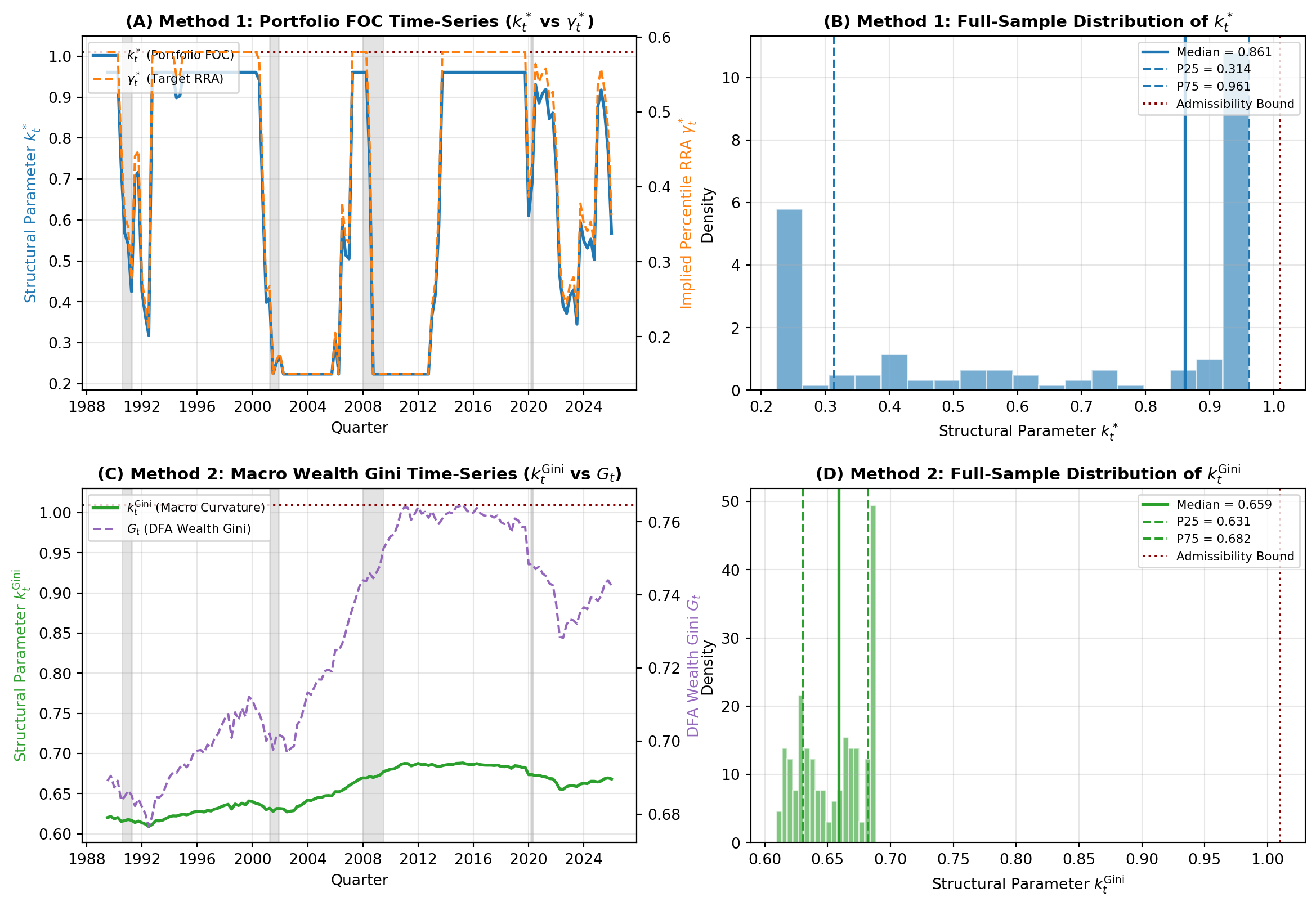
fig, axes = plt.subplots(2, 2, figsize=(13, 9))
fig.tight_layout(pad=4.5)

# Panel A: Method 1 Time-Series (Dual Axis + Recessions)
ax_a1 = axes[0, 0]
ax_a2 = ax_a1.twinx()

for i, (s, e) in enumerate(recessions):
    ax_a1.axvspan(s, e, color="gray", alpha=0.22, zorder=0, label="NBER Recession" if i == 0 else "")

p1, = ax_a1.plot(common_idx, k_star, color="#1f77b4", lw=2.0, zorder=2, label=r"$k_t^*$ (Portfolio FOC)")
p2, = ax_a2.plot(common_idx, gamma_star, color="#ff7f0e", lw=1.5, ls="--", zorder=2, label=r"$\gamma_t^*$ (Target RRA)")
ax_a1.axhline(1.0101, color="darkred", ls=":", lw=1.5, zorder=1, label="Limit (1.0101)")
ax_a1.set_title(r"(A) Method 1: Portfolio FOC Time-Series ($k_t^*$ vs $\gamma_t^*$)", fontsize=11, fontweight="bold")
ax_a1.set_xlabel("Quarter")
ax_a1.set_ylabel(r"Structural Parameter $k_t^*$", color="#1f77b4")
ax_a2.set_ylabel(r"Implied Percentile RRA $\gamma_t^*$", color="#ff7f0e")
ax_a1.grid(True, alpha=0.3)
lines_a = [p1, p2]
ax_a1.legend(lines_a, [l.get_label() for l in lines_a], loc="upper left", frameon=True, fontsize=8)

# Panel B: Method 1 Full-Sample Distribution
ax_b = axes[0, 1]
ax_b.hist(k_star, bins=18, density=True, color="#1f77b4", alpha=0.6, edgecolor="white")
ax_b.axvline(np.median(k_star), color="#1f77b4", lw=2.0, ls="-", label=f"Median = {np.median(k_star):.3f}")
ax_b.axvline(np.percentile(k_star, 25), color="#1f77b4", lw=1.5, ls="--", label=f"P25 = {np.percentile(k_star, 25):.3f}")
ax_b.axvline(np.percentile(k_star, 75), color="#1f77b4", lw=1.5, ls="--", label=f"P75 = {np.percentile(k_star, 75):.3f}")
ax_b.axvline(1.0101, color="darkred", ls=":", lw=1.5, label="Admissibility Bound")
ax_b.set_title(r"(B) Method 1: Full-Sample Distribution of $k_t^*$", fontsize=11, fontweight="bold")
ax_b.set_xlabel(r"Structural Parameter $k_t^*$")
ax_b.set_ylabel("Density")
ax_b.grid(True, alpha=0.3)
ax_b.legend(loc="upper right", frameon=True, fontsize=8)

# Panel C: Method 2 Time-Series (Dual Axis + Recessions)
ax_c1 = axes[1, 0]
ax_c2 = ax_c1.twinx()

for i, (s, e) in enumerate(recessions):
    ax_c1.axvspan(s, e, color="gray", alpha=0.22, zorder=0, label="NBER Recession" if i == 0 else "")

p3, = ax_c1.plot(common_idx, k_gini, color="#2ca02c", lw=2.0, zorder=2, label=r"$k_t^{\mathrm{Gini}}$ (Macro Curvature)")
p4, = ax_c2.plot(common_idx, gini_t, color="#9467bd", lw=1.5, ls="--", zorder=2, label=r"$G_t$ (DFA Wealth Gini)")
ax_c1.axhline(1.0101, color="darkred", ls=":", lw=1.5, zorder=1, label="Limit (1.0101)")
ax_c1.set_title(r"(C) Method 2: Macro Wealth Gini Time-Series ($k_t^{\mathrm{Gini}}$ vs $G_t$)", fontsize=11, fontweight="bold")
ax_c1.set_xlabel("Quarter")
ax_c1.set_ylabel(r"Structural Parameter $k_t^{\mathrm{Gini}}$", color="#2ca02c")
ax_c2.set_ylabel(r"DFA Wealth Gini $G_t$", color="#9467bd")
ax_c1.grid(True, alpha=0.3)
lines_c = [p3, p4]
ax_c1.legend(lines_c, [l.get_label() for l in lines_c], loc="upper left", frameon=True, fontsize=8)

# Panel D: Method 2 Full-Sample Distribution
ax_d = axes[1, 1]
ax_d.hist(k_gini, bins=18, density=True, color="#2ca02c", alpha=0.6, edgecolor="white")
ax_d.axvline(np.median(k_gini), color="#2ca02c", lw=2.0, ls="-", label=f"Median = {np.median(k_gini):.3f}")
ax_d.axvline(np.percentile(k_gini, 25), color="#2ca02c", lw=1.5, ls="--", label=f"P25 = {np.percentile(k_gini, 25):.3f}")
ax_d.axvline(np.percentile(k_gini, 75), color="#2ca02c", lw=1.5, ls="--", label=f"P75 = {np.percentile(k_gini, 75):.3f}")
ax_d.axvline(1.0101, color="darkred", ls=":", lw=1.5, label="Admissibility Bound")
ax_d.set_title(r"(D) Method 2: Full-Sample Distribution of $k_t^{\mathrm{Gini}}$", fontsize=11, fontweight="bold")
ax_d.set_xlabel(r"Structural Parameter $k_t^{\mathrm{Gini}}$")
ax_d.set_ylabel("Density")
ax_d.grid(True, alpha=0.3)
ax_d.legend(loc="upper right", frameon=True, fontsize=8)

plt.show()

Figure 1: Quarterly Calibration Dynamics and Full-Sample Distributions of Structural Curvature Parameter ($k_t$) with NBER Recession Shading

The empirical distributions confirm that both calibration routes produce parameter trajectories strictly bounded within the admissible domain $k_t \in (0, 1.0101)$, verifying Proposition 1 across expansions and recessions alike. Method 1 reveals countercyclical surges in curvature during NBER recessions (such as the 2008 Great Financial Crisis and 2020 COVID shock), reflecting heightened defensive risk aversion as equity allocations contract. Method 2 demonstrates a secular upward drift in curvature intensity driven by the long-run rise in US wealth concentration ($G_t$ rising from 0.68 in 1989 to 0.74 in 2026).

To analyze how historical variation in $k_t$ reshapes the representative utility curve and stochastic discount factor, Figure 2 plots the calibrated quartic utility function $u(x)$ and marginal utility $u'(x)$ evaluated across the empirical interquartile range (IQR: 25th, 50th, and 75th percentiles) of estimated $k_t^*$.

Code

# ---------------------------------------------------------
# 4. Figure 2: Utility Function and Pricing Kernel Bands
# ---------------------------------------------------------
x1, x2 = 0.50, 0.99
P1 = 1 - 2 * (x1 + x2) + 6 * x1 * x2  # 0.99

def u_func(x, k):
    Px = x**4 - 2 * (x1 + x2) * x**3 + 6 * x1 * x2 * x**2
    return k * Px + (1 - k * P1) * x

def u_prime_func(x, k):
    Qx = 4 * x**3 - 6 * (x1 + x2) * x**2 + 12 * x1 * x2 * x
    return k * Qx + (1 - k * P1)

x_grid = np.linspace(0, 1, 500)
k_p25 = float(np.percentile(k_star, 25))
k_med = float(np.median(k_star))
k_p75 = float(np.percentile(k_star, 75))

fig, (ax1, ax2) = plt.subplots(1, 2, figsize=(13, 5.5))
fig.tight_layout(pad=4.5)

# Panel A: Quartic Utility u(x)
ax1.plot(x_grid, x_grid, "k--", alpha=0.35, label=r"Egalitarian Benchmark ($u=x$)")
ax1.plot(x_grid, u_func(x_grid, k_med), color="#1f77b4", lw=2.2, label=f"Median $k = {k_med:.3f}$")
ax1.fill_between(x_grid, u_func(x_grid, k_p25), u_func(x_grid, k_p75), color="#1f77b4", alpha=0.20, label="IQR Band (P25–P75)")

for ax in (ax1, ax2):
    ax.axvline(x1, color="gray", ls=":", lw=1.2)
    ax.axvline(x2, color="gray", ls=":", lw=1.2)
    ax.grid(True, alpha=0.3)

ax1.set_title(r"(A) Calibrated Quartic Utility: $u(x)$", fontsize=11, fontweight="bold")
ax1.set_xlabel("Wealth Percentile ($x$)")
ax1.set_ylabel(r"Utility $u(x)$")
ax1.set_xlim(0, 1)
ax1.set_ylim(0, 1.05)
ax1.text(0.25, 0.35, "Working Class\n(Convex)", ha="center", fontsize=9, color="#2c3e50", style="italic")
ax1.text(0.75, 0.65, "Middle Class\n(Concave)", ha="center", fontsize=9, color="#2c3e50", style="italic")
ax1.text(0.97, 0.85, "Top 1%\n(Convex)", ha="right", fontsize=9, color="#2c3e50", style="italic")
ax1.legend(loc="upper left", frameon=True, fontsize=9)

# Panel B: Marginal Utility u'(x) (Pricing Kernel SDF Proxy)
ax2.plot(x_grid, u_prime_func(x_grid, k_med), color="#d62728", lw=2.2, label=f"Median $k = {k_med:.3f}$")
ax2.fill_between(x_grid, u_prime_func(x_grid, k_p25), u_prime_func(x_grid, k_p75), color="#d62728", alpha=0.20, label="IQR Band (P25–P75)")
ax2.axhline(1.0, color="k", ls="--", alpha=0.35, label=r"Linear Reference ($u'=1$)")

ax2.set_title(r"(B) Marginal Utility / Pricing Kernel Proxy: $u'(x)$", fontsize=11, fontweight="bold")
ax2.set_xlabel("Wealth Percentile ($x$)")
ax2.set_ylabel(r"Marginal Utility $u'(x)$")
ax2.set_xlim(0, 1)
ax2.text(0.25, 0.70, "Speculative Drop\n($u'' > 0$)", ha="center", fontsize=9, color="#8b0000", style="italic")
ax2.text(0.75, 1.12, "Defensive Elevation\n($u'' < 0$)", ha="center", fontsize=9, color="#8b0000", style="italic")
ax2.text(0.97, 0.75, "U-Shape\nTurnaround", ha="right", fontsize=9, color="#8b0000", style="italic")
ax2.legend(loc="lower left", frameon=True, fontsize=9)

plt.show()

Figure 2: Empirically Calibrated Quartic Utility Function $u(x)$ and Marginal Utility (Pricing Kernel Proxy) $u'(x)$ across Sample Quantiles

The resulting structural curves demonstrate that marginal utility $u'(x)$ endogenously generates the empirical U-shaped pricing kernel: dropping sharply through the working-class tier, rising and flattening across the defensive middle class, and rebounding at the top percentile. The interquartile band reveals that macroeconomic expansions and rising inequality amplify this curvature spread without violating global monotonicity.

4.3 4.3 Implications

The quartic utility function generates identical mathematical curvature ($u'' > 0$) at both tails of the wealth distribution. A superficial reading would classify both the working class and the ultra-rich as “risk-seeking.” This formal symmetry, however, conceals a qualitative asymmetry rooted in the market role each tier occupies.

4.3.1 Price Takers and Risk-Seeking at the Bottom

For agents below the median ($x < 0.50$), the price-taking assumption of standard portfolio theory holds without qualification. These households interact with financial markets through exchange-listed securities, mutual funds, and retail brokerage platforms where prices are publicly quoted and individually non-manipulable. The return distribution $F(R)$ is exogenous to their decisions. Within this fixed distributional environment, convex utility ($u'' > 0$) generates a rational preference for high-variance, positively skewed assets—lottery tickets, out-of-the-money call options, meme stocks, and speculative cryptoassets. This is a risk-seeking behavior in the classical sense: agents accept unfavorable expected values in exchange for the possibility of a discontinuous upward jump in percentile rank.

4.3.2 Price Makers and Rent-Seeking at the Top

For agents above the 99th percentile ($x \geq 0.99$), the price-taking assumption breaks down. The defining characteristic of ultra-high-net-worth capital is not merely its volume but its capacity to set terms. In pre-IPO financing rounds, the lead investor negotiates valuation caps, liquidation preferences, anti-dilution provisions, and board representation. In direct lending and private credit, the lender dictates covenants, collateral requirements, and pricing spreads. In distressed acquisitions, the acquirer determines the bid price in a thin, illiquid market with few competing participants. In each case, the return distribution is not passively received but actively constructed.

This distinction transforms the economic interpretation of the upper convex region. The working class, as price takers, exhibits risk-seeking behavior—accepting gambles within a given probability structure. The ultra-rich, as price makers, exhibits rent-seeking behavior—engineering probability structures that systematically favor their position. Both produce $u'' > 0$ in the reduced-form utility function, but the causal pathways diverge at the level of market microstructure.

4.3.3 Implications for the Exogenous DGP Assumption

Standard expected utility theory, and by extension the portfolio optimization framework employed in Section 3.5, presupposes that the data generating process (DGP) for asset returns is exogenous to any individual agent’s decisions. This assumption is empirically defensible for the bottom 99% of the wealth distribution, where individual portfolio choices exert negligible price impact. For the top 1%, however, concentrated capital flows materially affect asset valuations, deal structures, and secondary market liquidity. The return distribution faced by an ultra-rich household becomes a function of its own allocation decisions: $F(R \mid a, x)$ rather than $F(R)$.

This endogeneity does not invalidate the quartic utility model as a descriptive device—the convex-concave-convex curvature pattern faithfully captures the observed cross-sectional variation in revealed risk attitudes. It does, however, constrain the normative and causal interpretation of the upper convex region. The calibration strategy of Section 3.5, which identifies $k$ from middle-class portfolio behavior at $x^* = 0.70$, operates entirely within the price-taking regime and retains full theoretical validity. Extrapolating the same exogenous-DGP framework to the top percentile conflates structural market power with preference-driven risk appetite. A complete theory of ultra-rich investment behavior would require supplementing the percentile utility model with a game-theoretic or mechanism design framework in which the agent’s action set includes not only portfolio weights but also the contractual terms that define the return distribution itself.

4.3.4 Balance Sheet Anatomy across Wealth Tiers

To provide concrete microstructural foundations for the asymmetric risk behaviors modeled above, Figure 3 examines the cross-sectional balance sheet compositions across the four DFA wealth tiers for the latest available snapshot (2026:Q1).

The Federal Reserve DFA accounting identity strictly satisfies:

\[\text{Total Net Worth} \equiv \text{Nonfinancial Assets} + \text{Financial Assets} - \text{Total Liabilities}\]

Defining Net Financial Assets as financial claims net of all liabilities ($\text{Net Financial Assets} \equiv \text{Financial Assets} - \text{Total Liabilities}$), dividing through by Total Net Worth yields the structural balance-sheet partition:

\[1 \equiv \frac{\text{Nonfinancial Assets}}{\text{Net Worth}} + \frac{\text{Net Financial Assets}}{\text{Net Worth}}\]

Code

import os
import numpy as np
import pandas as pd
import matplotlib.pyplot as plt

# ---------------------------------------------------------
# Ingestion of Balance Sheet Quantities (2026:Q1)
# ---------------------------------------------------------
tier_codes = {
    "Top 1%\n(99th–100th)": {
        "nfa": "WFRBLT01001", "fa": "WFRBLT01004", "liab": "WFRBLT01019", "nw": "WFRBLT01026", "eq": "WFRBLT01014"
    },
    "90th to 99th\nPercentiles": {
        "nfa": "WFRBLN09028", "fa": "WFRBLN09031", "liab": "WFRBLN09046", "nw": "WFRBLN09053", "eq": "WFRBLN09041"
    },
    "50th to 90th\nPercentiles": {
        "nfa": "WFRBLN40055", "fa": "WFRBLN40058", "liab": "WFRBLN40073", "nw": "WFRBLN40080", "eq": "WFRBLN40068"
    },
    "Bottom 50%\n(1st–50th)": {
        "nfa": "WFRBLB50082", "fa": "WFRBLB50085", "liab": "WFRBLB50100", "nw": "WFRBLB50107", "eq": "WFRBLB50095"
    }
}

labels = list(tier_codes.keys())
eq_fa_shares = []
nfa_nw_shares = []
net_fa_nw_shares = []

for label, s in tier_codes.items():
    nfa_val = get_fred_data(s["nfa"]).iloc[-1]
    fa_val = get_fred_data(s["fa"]).iloc[-1]
    liab_val = get_fred_data(s["liab"]).iloc[-1]
    nw_val = get_fred_data(s["nw"]).iloc[-1]
    eq_val = get_fred_data(s["eq"]).iloc[-1]
    
    net_fa_val = fa_val - liab_val
    eq_fa_shares.append((eq_val / fa_val) * 100.0)
    nfa_nw_shares.append((nfa_val / nw_val) * 100.0)
    net_fa_nw_shares.append((net_fa_val / nw_val) * 100.0)

# ---------------------------------------------------------
# Figure 3: Dual-Panel Comparison
# ---------------------------------------------------------
fig, (ax1, ax2) = plt.subplots(1, 2, figsize=(13, 5.5))
fig.tight_layout(pad=4.5)
x_pos = np.arange(len(labels))
bar_width = 0.55

# Panel A: Equity & Mutual Fund Share of Financial Assets
bars1 = ax1.bar(x_pos, eq_fa_shares, width=bar_width, color="#1f4e79", edgecolor="white", lw=1.2)
ax1.set_xticks(x_pos)
ax1.set_xticklabels(labels, fontsize=9)
ax1.set_ylabel("Equity & Mutual Funds / Financial Assets (%)", fontsize=10)
ax1.set_ylim(0, 68)
ax1.set_title("(A) Equity Share of Financial Assets (2026:Q1)", fontsize=11, fontweight="bold")
ax1.grid(True, axis="y", alpha=0.3)

for bar, val in zip(bars1, eq_fa_shares):
    ax1.text(bar.get_x() + bar.get_width() / 2, val + 1.2, f"{val:.1f}%", ha="center", va="bottom", fontsize=9, fontweight="bold")

# Panel B: Stacked Net Financial Assets vs Real Assets as % of Net Worth
for i in range(len(labels)):
    if net_fa_nw_shares[i] >= 0:
        ax2.bar(x_pos[i], nfa_nw_shares[i], width=bar_width, color="#1f4e79", edgecolor="white", lw=1.2)
        ax2.bar(x_pos[i], net_fa_nw_shares[i], bottom=nfa_nw_shares[i], width=bar_width, color="#7baaf7", edgecolor="white", lw=1.2)
    else:
        ax2.bar(x_pos[i], nfa_nw_shares[i], width=bar_width, color="#1f4e79", edgecolor="white", lw=1.2)
        ax2.bar(x_pos[i], net_fa_nw_shares[i], bottom=0, width=bar_width, color="#7baaf7", edgecolor="white", lw=1.2)

ax2.axhline(0, color="black", lw=1.0)
ax2.axhline(100, color="gray", ls="--", lw=1.0, alpha=0.7)
ax2.set_xticks(x_pos)
ax2.set_xticklabels(labels, fontsize=9)
ax2.set_ylabel("% of Group Net Worth", fontsize=10)
ax2.set_ylim(-85, 195)
ax2.set_title("(B) Balance Sheet Partition: Real vs Net Financial Assets (2026:Q1)", fontsize=11, fontweight="bold")
ax2.grid(True, axis="y", alpha=0.3)

from matplotlib.patches import Patch
legend_items = [
    Patch(facecolor="#7baaf7", edgecolor="white", label="Net Financial Assets (Financial Assets − Liabilities) / NW"),
    Patch(facecolor="#1f4e79", edgecolor="white", label="Real Assets (Nonfinancial Assets) / NW"),
    plt.Line2D([0], [0], color="gray", ls="--", label="100% Net Worth Bound")
]
ax2.legend(handles=legend_items, loc="upper center", bbox_to_anchor=(0.5, -0.16), ncol=3, frameon=True, fontsize=8)

plt.show()

Figure 3: Cross-Sectional Balance Sheet Anatomy across Wealth Percentiles (2026:Q1 Snapshot)

The empirical cross-section in Figure 3 reveals two critical balance-sheet realities that reinforce our theoretical model:

Capital Concentration at the Top (Panel A): Equities and mutual fund shares constitute 57.1% of liquid financial wealth for the top 1% and 40.5% for the 90th–99th percentile, contrasting sharply with the defensive 17%–19% allocations observed across the middle and lower tiers.
Negative Net Financial Wealth of the Bottom 50% (Panel B): While the top 1% holds 86.2% of its net worth in net financial claims, the bottom 50% maintains a negative net financial asset position ($-62.6\%$ of net worth, where liabilities of $6.08 trillion exceed financial assets of $3.41 trillion). Consequently, real assets (primarily residential housing and consumer durables) constitute 162.6% of working-class net worth. This acute leverage exposure leaves lower-tier households structurally foreclosed from linear capital-accumulation paths, driving the rational pursuit of high-variance, convex payoff structures documented in Section 4.3.

5 5. Conclusion

This paper establishes that heterogeneous risk preferences and pricing kernel non-monotonicities can be reconciled as structural outcomes of household optimization over relative wealth percentiles, $x \in [0, 1]$. By shifting the primitive domain from absolute wealth to relative rank, the quartic utility specification avoids wealth-scale distortion under aggregate economic growth and eliminates the computational burden of high-dimensional dynamic programming. The single curvature parameter $k$ provides an analytical bridge linking microeconomic portfolio allocations to aggregate macroeconomic wealth concentration.

A key methodological strength of the framework is anchoring the structural inflection points to the empirical distribution boundaries, $x_1 = 0.50$ and $x_2 = 0.99$. Rather than treating these coordinates as free parameters—which would introduce identification fragility and risk overfitting—they directly reflect the institutional wealth strata standardized by the Federal Reserve DFA and the World Inequality Database. This structural choice reduces the estimation problem to a single identifiable parameter $k$, guarantees global monotonicity ($u'(x) > 0$) across empirical regimes under Proposition 1, and offers a natural comparative statics instrument to evaluate secular shifts such as a shrinking middle class.

The primary theoretical implication is the economic decoupling of the two convex tails. While standard expected utility frameworks treat convexity symmetrically, our analysis demonstrates that identical curvature signs ($u'' > 0$) reflect contrasting market roles: price-taking risk-seeking at the bottom versus price-making rent extraction at the top. This distinction highlights the boundary of the exogenous data generating process assumption, which holds across the broad public market but fails at the extreme upper tail where capital concentrates price-setting power. Macroeconomic policies aimed at market stability must therefore separate distributional measures that restore mobility for the bottom from structural competition policies that discipline capital dominance at the top.

6 Appendix A. Mathematical Derivations and Proofs

6.1 A.1 Derivation of the Quartic Utility Specification

Starting from the specified quadratic curvature in Section 3.2:

\[u''(x) = 12k (x - x_1)(x - x_2) = 12k \left( x^2 - (x_1 + x_2)x + x_1 x_2 \right)\]

where $k > 0$ denotes the curvature intensity parameter. Integrating $u''(x)$ with respect to $x$ yields the marginal utility function $u'(x)$:

\[u'(x) = 12k \left( \frac{x^3}{3} - \frac{x_1 + x_2}{2}x^2 + x_1 x_2 x \right) + C_1 = k Q(x) + C_1\]

where the cubic polynomial basis $Q(x)$ is defined as:

\[Q(x) \equiv 4x^3 - 6(x_1 + x_2)x^2 + 12x_1 x_2 x\]

and $C_1$ is a constant of integration representing marginal utility at the lower boundary, $u'(0) = C_1$.

Integrating $u'(x)$ with respect to $x$ provides the total utility function:

\[u(x) = k \left( x^4 - 2(x_1 + x_2)x^3 + 6x_1 x_2 x^2 \right) + C_1 x + C_0 = k P(x) + C_1 x + C_0\]

where the quartic polynomial basis $P(x)$ is defined as:

\[P(x) \equiv x^4 - 2(x_1 + x_2)x^3 + 6x_1 x_2 x^2\]

Enforcing the lower boundary normalization $u(0) = 0$ requires:

\[u(0) = C_0 = 0\]

Applying the terminal normalization constraint $u(1) = 1$ uniquely determines the integration constant $C_1$ as an affine function of $k$:

\[u(1) = k P(1) + C_1 = 1 \implies C_1(k) = 1 - k P(1)\]

where:

\[P(1) = 1 - 2(x_1 + x_2) + 6x_1 x_2\]

Substituting $C_1(k)$ back into the primitive equations establishes the closed-form expressions for total and marginal utility:

\[u(x) = k P(x) + \left( 1 - k P(1) \right) x\]

\[u'(x) = k Q(x) + \left( 1 - k P(1) \right)\]

6.2 A.2 Proof of Proposition 1 (Global Monotonicity and Admissibility)

Proof. Non-satiation requires $u'(x) > 0$ for all $x \in [0, 1]$ (Section 3.3). Differentiating $u'(x)$ gives $u''(x) = 12k(x - x_1)(x - x_2)$. For $k > 0$ and $0 < x_1 < x_2 < 1$:

$u''(x) > 0$ on $[0, x_1) \cup (x_2, 1]$, indicating that $u'(x)$ is strictly increasing on these subintervals.
$u''(x) < 0$ on $(x_1, x_2)$, indicating that $u'(x)$ is strictly decreasing on this subinterval.

Consequently, $u'(x)$ attains its unique internal local minimum at $x = x_2$. Global monotonicity over the compact interval $[0, 1]$ holds if and only if the boundary minimum and internal minimum remain strictly positive:

\[\min_{x \in [0, 1]} u'(x) = \min \left\{ u'(0), u'(x_2) \right\} > 0\]

Evaluating $Q(x)$ at $x = x_2$:

\[Q(x_2) = 4x_2^3 - 6(x_1 + x_2)x_2^2 + 12x_1 x_2^2 = x_2^2 \left( 6x_1 - 2x_2 \right)\]

Evaluating marginal utility at the local minimum $x_2$:

\[u'(x_2) = k Q(x_2) + 1 - k P(1) = 1 - k \left[ P(1) - x_2^2 (6x_1 - 2x_2) \right]\]

Defining $\Delta(x_1, x_2) \equiv P(1) - x_2^2 (6x_1 - 2x_2)$, the condition $u'(x_2) > 0$ becomes:

\[1 - k \Delta(x_1, x_2) > 0\]

For empirical benchmark parameters $x_1 = 0.50$ and $x_2 = 0.99$:

\[P(1) = 1 - 2(0.50 + 0.99) + 6(0.50)(0.99) = 1 - 2.98 + 2.97 = 0.99\]

\[x_2^2 (6x_1 - 2x_2) = (0.99)^2 \left( 6(0.50) - 2(0.99) \right) = 0.9801 (3.00 - 1.98) = 0.9801 \times 1.02 = 0.999702\]

\[\Delta(0.50, 0.99) = 0.99 - 0.999702 = -0.009702 < 0\]

Substituting $\Delta$ into the expression for $u'(x_2)$:

\[u'(x_2) = 1 - k (-0.009702) = 1 + 0.009702 k > 1 > 0 \quad \forall k > 0\]

Because $\Delta < 0$, the interior minimum $u'(x_2)$ exceeds 1 for all positive values of $k$, meaning the local minimum never binds. The binding upper bound on $k$ is dictated solely by the lower boundary condition:

\[u'(0) = C_1(k) = 1 - k P(1) > 0 \implies k < \frac{1}{P(1)} = \frac{1}{0.99} \approx 1.0101\]

Together with the curvature requirement $k > 0$, the admissible parameter range is uniquely characterized as $k \in (0, 1.0101)$. $\blacksquare$

7 Appendix B. Calibration Derivations and Mappings

7.1 B.1 Derivation of the Closed-Form Portfolio Estimator

This section details the algebraic steps connecting middle-class portfolio allocations in Section 3.5 to the curvature parameter $k_t^*$.

From Section 3, the Arrow-Pratt coefficient of relative risk aversion in percentile space is defined as:

\[\gamma(x^*; k) = - \frac{u''(x^*; k)}{u'(x^*; k)} = - \frac{12k(x^* - x_1)(x^* - x_2)}{k Q(x^*) + C_1(k)}\]

Substituting $C_1(k) = 1 - k P(1)$ from Appendix A.1 yields:

\[u'(x^*; k) = 1 + k \left( Q(x^*) - P(1) \right)\]

Equating the model-implied measure to the empirical target $\gamma^*_t = \frac{\mathbb{E}_t[R_m - R_f]}{\sigma_{m,t}^2 \cdot w(x^*)_t}$ produces:

\[- 12k (x^* - x_1)(x^* - x_2) = \gamma^*_t \left[ 1 + k \left( Q(x^*) - P(1) \right) \right]\]

Rearranging terms to isolate $k$:

\[k \left[ - 12(x^* - x_1)(x^* - x_2) - \gamma^*_t \left( Q(x^*) - P(1) \right) \right] = \gamma^*_t\]

Solving for $k_t^*$ provides the general closed-form estimator:

\[k_t^* = \frac{\gamma^*_t}{- 12(x^* - x_1)(x^* - x_2) - \gamma^*_t \left( Q(x^*) - P(1) \right)}\]

For benchmark inflection coordinates $x_1 = 0.50$, $x_2 = 0.99$, and middle-class representative coordinate $x^* = 0.70$:

\[(x^* - x_1)(x^* - x_2) = (0.70 - 0.50)(0.70 - 0.99) = (0.20)(-0.29) = -0.058\]

\[-12(x^* - x_1)(x^* - x_2) = -12(-0.058) = 0.696\]

Evaluating the polynomial basis coefficients:

\[P(1) = 1 - 2(1.49) + 6(0.495) = 0.99\]

\[Q(0.70) = 4(0.70)^3 - 6(1.49)(0.70)^2 + 12(0.495)(0.70) = 1.372 - 4.3806 + 4.158 = 1.1494\]

\[Q(0.70) - P(1) = 1.1494 - 0.99 = 0.1594\]

Substituting these constants into the general expression yields the simplified operational estimator:

\[k_t^* = \frac{\gamma^*_t}{0.696 - 0.1594 \cdot \gamma^*_t}\]

7.2 B.2 Derivation of the Macroeconomic Wealth Gini Mapping

This section details the definite integral calculations linking aggregate wealth concentration to the curvature parameter in Section 3.5.

The macroeconomic welfare gap condition is:

\[\int_0^1 \left( x - u(x) \right) dx = \theta \cdot G_t\]

Substituting $u(x) = k P(x) + (1 - k P(1))x$:

\[\int_0^1 \left( x - u(x) \right) dx = \int_0^1 \left[ x - k P(x) - (1 - k P(1))x \right] dx = k \left[ P(1) \int_0^1 x \, dx - \int_0^1 P(x) \, dx \right]\]

Evaluating the definite integrals:

\[\int_0^1 x \, dx = \left[ \frac{x^2}{2} \right]_0^1 = \frac{1}{2}\]

\[\int_0^1 P(x) \, dx = \int_0^1 \left( x^4 - 2(x_1 + x_2)x^3 + 6x_1 x_2 x^2 \right) dx = \left[ \frac{x^5}{5} - \frac{x_1 + x_2}{2}x^4 + 2x_1 x_2 x^3 \right]_0^1 = \frac{1}{5} - \frac{x_1 + x_2}{2} + 2 x_1 x_2 \equiv I_P\]

Evaluating $I_P$ at empirical benchmark coordinates $x_1 = 0.50$ and $x_2 = 0.99$:

\[I_P = 0.20 - \frac{1.49}{2} + 2(0.495) = 0.20 - 0.745 + 0.99 = 0.445\]

The difference in the bracket is:

\[\frac{1}{2} P(1) - I_P = \frac{1}{2}(0.99) - 0.445 = 0.495 - 0.445 = 0.050\]

Substituting this into the welfare gap equality yields:

\[0.050 \cdot k = \theta \cdot G_t \implies k_t^{\text{Gini}} = \frac{\theta \cdot G_t}{0.050} = 20 \cdot \theta \cdot G_t\]

References

Aiyagari, S. Rao. 1994. “Uninsured Idiosyncratic Risk and Aggregate Saving.” The Quarterly Journal of Economics 109 (3): 659–84.

Aı̈t-Sahalia, Yacine, and Andrew W. Lo. 1998. “Nonparametric Estimation of State-Price Densities Implicit in Financial Asset Prices.” The Journal of Finance 53 (2): 499–547.

Aı̈t-Sahalia, Yacine, Yubo Wang, and Francis Yared. 2001. “Do Option Markets Correctly Price the Probabilities of Movement of the Underlying Asset?” Journal of Econometrics 102 (1): 67–110.

Beare, Brendan K. 2011. “Measure Preserving Derivatives and the Pricing Kernel Puzzle.” Journal of Mathematical Economics 47 (6): 689–97.

Becker, Gary S., Kevin M. Murphy, and Iván Werning. 2005. “The Equilibrium Distribution of Income and the Market for Status.” Journal of Political Economy 113 (2): 282–310.

Bewley, Truman F. 1986. “Stationary Monetary Equilibrium with a Continuum of Independently Fluctuating Consumers.” In Contributions to Mathematical Economics in Honor of gérard Debreu, edited by Werner Hildenbrand and Andreu Mas-Colell. North-Holland.

Bliss, Robert R., and Nikolaos Panigirtzoglou. 2004. “Option-Implied Risk Aversion Estimates.” The Journal of Finance 59 (1): 407–46.

Chen, Luyang, Markus Pelger, and Jason Zhu. 2024. “Deep Learning in Asset Pricing.” Management Science 70 (2): 714–50.

Corak, Miles. 2013. “Income Inequality, Equality of Opportunity, and Intergenerational Mobility.” Journal of Economic Perspectives 27 (3): 79–102.

Friedman, Milton, and L. J. Savage. 1948. “The Utility Analysis of Choices Involving Risk.” Journal of Political Economy 56 (4): 279–304.

Gu, Shihao, Bryan Kelly, and Dacheng Xiu. 2021. “Autoencoder Asset Pricing Models.” Journal of Econometrics 222 (1): 429–50.

Guvenen, Fatih, Fatih Karahan, Serdar Ozkan, and Jae Song. 2021. “What Do Data on Millions of U.S. Workers Reveal about Lifecycle Earnings Dynamics?” Econometrica 89 (5): 2303–39.

Hartley, Roger, and Lisa Farrell. 2002. “Can Expected Utility Theory Explain Gambling?” The American Economic Review 92 (3): 613–24.

Huggett, Mark. 1993. “The Risk-Free Rate in Heterogeneous-Agent Incomplete-Insurance Economies.” Journal of Economic Dynamics and Control 17 (5–6): 953–69.

Jackwerth, Jens Carsten. 2000. “Recovering Risk Aversion from Option Prices and Realized Returns.” The Review of Financial Studies 13 (2): 433–51.

Kaplan, Greg, Benjamin Moll, and Giovanni L. Violante. 2018. “Monetary Policy According to HANK.” American Economic Review 108 (3): 697–743.

Kraus, Alan, and Robert H. Litzenberger. 1976. “Skewness Preference and the Valuation of Risk Assets.” The Journal of Finance 31 (4): 1085–100.

Krueger, Alan B. 2012. The Rise and Consequences of Inequality in the United States. Speech at the Center for American Progress, Washington D.C.

Ray, Debraj, and Arthur Robson. 2012. “Status, Intertemporal Choice, and Risk-Taking.” Econometrica 80 (4): 1505–31.

Robson, Arthur J. 1992. “Status, the Distribution of Wealth, Private and Social Attitudes to Risk.” Econometrica 60 (4): 837–57.

Rosenberg, Joshua V., and Robert F. Engle. 2002. “Empirical Pricing Kernels.” Journal of Financial Economics 64 (3): 341–72.

Scott, Robert C., and Philip A. Horvath. 1980. “On the Direction of Preference for Moments of Higher Order Than the Variance.” The Journal of Finance 35 (4): 915–19.