Beyond Heuristic Projections of Bitcoin

Quantitative Instability and Bias in Long-Horizon Price Simulations

Data
Theory
Author

GitSAM

Published

October 28, 2026

Keywords

Monte Carlo Simulation, Bitcoin, Model Bias

Introduction

Long-term price projections for Bitcoin have increasingly penetrated both retail and institutional discourse, frequently popularized by industry practitioners through heuristic simulation models. A prominent example is the Monte Carlo framework advanced by on-chain analyst Willy Woo, which projects long-horizon terminal prices via repeated path generation calibrated to historical series. While such analyses provide accessible quantitative narratives, they routinely rely on critical empirical simplifications: the implicit assumption of weak stationarity across non-stationary series, heuristic parameter calibrations of drift (\(\mu\)) and volatility (\(\sigma\)), and an unadjusted reliance on Bitcoin’s early high-growth trajectory. Consequently, these models suffer from severe sample selection bias and survivorship bias, often confounding macroeconomic liquidity expansions with intrinsic asset dynamics while introducing non-trivial risks of data snooping and spurious regression.

To bridge the gap between heuristic industry practices and rigorous quantitative finance, this paper examines the path dependency and parametric instability inherent in historical data-driven projections. Specifically, we formalize the extent to which arbitrary lookback window selection (\(T_b\)) and untested distribution assumptions distort simulated future price distributions across lookforward horizons (\(T_f\)).

Our contributions are threefold:

  1. Parametric Sensitivity Analysis (GBM): We evaluate the stability of sample drift (\(\hat{\mu}\)) and volatility (\(\hat{\sigma}\)) under varying historical cut-off regimes (\(T_{\text{origin}}\)) and window lengths (\(T_b\)), proving that continuous compounding under Euler-Maruyama discretization generates explosive path divergences due to historical drift instability.
  2. Semi-Parametric & Non-Parametric Re-sampling (MBB): We implement a Moving Block Bootstrap (MBB) framework to preserve empirical volatility clustering and heavy-tailed innovations without Gaussian constraints, further benchmarking it against a semi-parametric additive decomposition that couples power-law trend damping, a halving cycle harmonic oscillator (\(T_{\text{half\_life}}\)), and a stationary autoregressive residual filter.
  3. Systematic Characterization of Forecast Bias: We introduce empirical metrics—namely the median forecast bias (\(\text{Bias}_{T_f}\)) and empirical coverage probability—to quantify how historical selection choices systematically induce structural bullish bias at market peaks, downward collapse bias at market troughs, and residual slope overhang in global power-law extrapolations.

Data

Mathematical Notations

Symbol Description Unit / Domain
\(t\) 제네시스 블록(Genesis Block, 2009-01-03) 기준 경과 일수 \(t \in \mathbb{N}\) (Days)
\(P_t\) 시점 \(t\)의 일별 자산 참조 종가(Reference Closing Price) USD
\(p_t\) 시점 \(t\)의 자연로그 가격 (\(\ln P_t\)) Real scalar
\(r_t\) 시점 \(t\)의 일간 연속복리 로그 수익률 (\(p_t - p_{t-1}\)) Real scalar
\(T_{\text{origin}}\) 모형 적합 및 표본 추출의 기준 시점 (Cut-off Point) YYYY-MM-DD (Date)
\(T_b\) 과거 관측 창(Lookback Window) 길이 Days (365, 730, 1460, All)
\(T_f\) 미래 예측 및 시뮬레이션 지평(Lookforward Horizon) Days (365, 1460)
\(T_{\text{half\_life}}\) 비트코인 블록 보상 반감 주기 (Halving Cycle Period) Days (1400, 1460, 1500)
\(\Delta t\) 이산 시간 간격 (1일 기준 \(1/365\)) Years
\(\mu, \sigma\) 일간 기대 수익률(Daily Drift) 및 변동성(Daily Volatility) Real scalars
\(\mu_{\text{ann}}, \sigma_{\text{ann}}\) 연율화 기대 수익률(Annualized Drift) 및 변동성(Annualized Volatility) Real scalars
\(L\) 이동 블록 부트스트랩(MBB) 블록 길이(Block Length) Days (10, 30, 60, 90)
\(\gamma\) 반감기 순환 진폭 감쇠 계수(Cycle Damping Factor) Real scalar (0.0, 0.25, 0.50)
\(\rho\) 구조적 잔차의 1차 자기회귀 평균회귀 계수(AR(1) Persistence) Real scalar \(\rho \in (0, 1)\)
\(M\) 몬테카를로 시뮬레이션 경로 반복 횟수 (Monte Carlo Paths) Integer (\(M = 10,000\))
\(m\) \(m\)번째 시뮬레이션 경로 인덱스 \(m \in \{1, 2, \dots, M\}\)

Primary Market Time Series

분석 대상 시계열은 CoinMetrics Community API를 통해 수집한 비트코인 일별 종가(Reference Rate Close Price, \(P_t\))이다. 단일 거래소의 유동성 공백(Liquidity Gap)이나 이상 호가 왜곡을 배제하기 위해 거래량 가중 중앙값(Volume-Weighted Median) 기반의 기관급 집계 시계열을 채택하며, 관측 구간은 2010년 7월 18일(\(t = 561\))부터 현재 시점(2026년 10월 27일, \(t = 6,506\))까지이다.

자연로그 가격 \(p_t = \ln P_t\) 및 연속복리 일간 로그 수익률(Log Return) \(r_t = p_t - p_{t-1}\) 시계열을 산출하고, 비트코인 제네시스 블록 생성일인 2009년 1월 3일을 기준점(\(t = 0\))으로 설정하여 정수형 경과 일수 \(t \in \mathbb{N}\)에 매핑한다.

CoinMetrics Community API v4는 기본 호출 시 최근 100일 분량만 반환하는 역방향 페이징(paging_from=end)을 기본값으로 취한다. 2010년 7월 18일 최초 관측일부터 현재까지의 전 구간 시계열을 단일 요청으로 수집하기 위해 정방향 페이징 파라미터(paging_from=start&page_size=10000)를 명시한다.

https://community-api.coinmetrics.io/v4/timeseries/asset-metrics?assets=btc&metrics=PriceUSD&frequency=1d&paging_from=start&page_size=10000

Halving Cycle Period Calibration (\(T_{\text{half\_life}}\))

준모수(Semi-parametric) 분해 모형의 주기적 순환 성분(Cyclical Component, \(c(t)\)) 추정에 반영할 비트코인 블록 보상 반감기(Halving) 확정 이력과 주기 통계량은 다음과 같다.

Halving Event Block Height Confirmed Date Elapsed Days from Prior
Genesis Block 0 2009-01-03 -
1st Halving 210,000 2012-11-28 1,425 days
2nd Halving 420,000 2016-07-09 1,319 days
3rd Halving 630,000 2020-05-11 1,402 days
4th Halving 840,000 2024-04-20 1,440 days
  • 실증 관측 범위(Empirical Range): \([1,319, \, 1,440]\) 일
  • 표본 평균 점추정치(Point Estimate): \(\bar{T}_{\text{half\_life}} \approx 1,396.5\) 일 (약 3.82년)
  • 프로토콜 이론치(Theoretical Target): \(210,000 \times 10 \text{ min} = 2,100,000 \text{ min} = 1,458.33\) 일 (약 4.0년)

네트워크 전체 연산 능력(Hashrate)이 장기 우상향함에 따라 2,016블록 단위의 난이도 조정(Difficulty Adjustment) 주기 내 평균 블록 생성 시간이 목표치인 10분보다 단축되는 경향이 존재한다. 실제 실현된 반감 주기는 이론치(1,458~1,460일)보다 짧은 구간에서 형성되므로, 그리드 탐색(Grid Search)의 \(T_{\text{half\_life}}\) 후보군은 실측 범위와 이론치를 포괄하는 \(\{1400, 1460, 1500\}\)일로 설정한다.

Reference Origins (\(T_{\text{origin}}\)) for Regime Stress Testing

거시 체제 전환(Regime Shift)과 모수 추정의 경로 의존성(Path Dependency)을 검증하기 위해, 과거 시장의 뚜렷한 과열 및 침체 국면을 대변하는 4개의 전환점을 기준 시점(\(T_{\text{origin}}\))으로 지정한다.

Cut-off Type Reference Date (\(T_{\text{origin}}\)) Market Regime Description
Bull Market Peak (Cycle 2) 2017-12-17 초기 글로벌 리테일 과열(FOMO) 폭발 및 파생상품(CME 선물) 상장 직전 고점
Bear Market Trough (Cycle 2) 2018-12-15 장기 유동성 고갈 및 채굴자 항복(Capitulation) 매도 국면 저점
Bull Market Peak (Cycle 3) 2021-11-10 제로 금리 양적완화(QE) 유동성 확장 및 기관 자금 유입 정점
Bear Market Trough (Cycle 3) 2022-11-21 시스템적 디레버리징(FTX 파산 사태) 및 통화 긴축 국면 저점

각 \(T_{\text{origin}}\) 시점에서 과거 관측 창(Lookback Window) \(T_b \in \{365, 730, 1460, \text{All}\}\)를 역방향으로 적용하여 모수를 추정한다. 기준 국면(고점 대비 저점)과 표본 관측 길이가 장기 시뮬레이션 궤적에 부여하는 표본 선택 편향(Sample Selection Bias)을 통제된 환경에서 분리해 낸다.

Code
import os
import requests
import pandas as pd
import numpy as np
import matplotlib.pyplot as plt
import scipy.stats as stats
import statsmodels.tsa.stattools as smt

# 1. 데이터 수집 및 로컬 캐싱
cache_path = "crypto_btc.csv"
if not os.path.exists(cache_path):
    url = "https://community-api.coinmetrics.io/v4/timeseries/asset-metrics?assets=btc&metrics=PriceUSD&frequency=1d&paging_from=start&page_size=10000"
    res = requests.get(url, timeout=30).json()
    raw_df = pd.DataFrame(res["data"])
    raw_df["date"] = pd.to_datetime(raw_df["time"]).dt.tz_localize(None)
    raw_df["PriceUSD"] = raw_df["PriceUSD"].astype(float)
    raw_df = raw_df.sort_values("date").reset_index(drop=True)
    genesis = pd.Timestamp("2009-01-03")
    raw_df["t"] = (raw_df["date"] - genesis).dt.days
    raw_df["p_t"] = np.log(raw_df["PriceUSD"])
    raw_df["r_t"] = raw_df["p_t"].diff()
    raw_df[["date", "t", "PriceUSD", "p_t", "r_t"]].to_csv(cache_path, index=False)

df = pd.read_csv(cache_path)
df["date"] = pd.to_datetime(df["date"])

# 2. 반감기 및 체제 기준 시점 정의
halvings = [
    pd.Timestamp("2012-11-28"),
    pd.Timestamp("2016-07-09"),
    pd.Timestamp("2020-05-11"),
    pd.Timestamp("2024-04-20")
]

origins = {
    "Peak (Cycle 2)": (pd.Timestamp("2017-12-17"), "crimson"),
    "Trough (Cycle 2)": (pd.Timestamp("2018-12-15"), "dodgerblue"),
    "Peak (Cycle 3)": (pd.Timestamp("2021-11-10"), "darkred"),
    "Trough (Cycle 3)": (pd.Timestamp("2022-11-21"), "navy")
}

# 3. 롤링 연율화 드리프트 및 변동성 계산
dt = 1.0 / 365.0
windows = [365, 730, 1460]
for w in windows:
    roll_mean = df["r_t"].rolling(w).mean()
    roll_vol = df["r_t"].rolling(w).std()
    ann_vol = roll_vol / np.sqrt(dt)
    ann_drift = (roll_mean / dt) + 0.5 * (ann_vol ** 2)
    df[f"drift_{w}"] = ann_drift
    df[f"vol_{w}"] = ann_vol

# 4. 시각화 (Panel A: 로그 가격 및 기준점, Panel B: 롤링 모수 비정상성)
plt.style.use("seaborn-v0_8-whitegrid" if "seaborn-v0_8-whitegrid" in plt.style.available else "default")
fig, (ax1, ax2) = plt.subplots(2, 1, figsize=(11, 8.5), sharex=True, gridspec_kw={"height_ratios": [1.2, 1]})

# Panel A
ax1.plot(df["date"], df["p_t"], color="#2c3e50", lw=1.3, label=r"Log Price $p_t = \ln P_t$")
for i, h in enumerate(halvings, 1):
    ax1.axvline(h, color="gray", linestyle="--", alpha=0.7, lw=1.0)
    ax1.text(h, -2.1, f"Halving {i}", rotation=90, va="bottom", ha="right", fontsize=8, color="dimgray")

for label, (origin_date, col) in origins.items():
    p_val = df.loc[df["date"] == origin_date, "p_t"].values
    if len(p_val) > 0:
        ax1.scatter(origin_date, p_val[0], color=col, s=45, zorder=5, label=f"Origin: {label}")

ax1.set_title("Bitcoin Empirical Dynamics: Log Price Trajectory and Reference Regimes", fontsize=11, fontweight="bold")
ax1.set_ylabel("Log Price (USD)", fontsize=10)
ax1.legend(loc="upper left", frameon=True, fontsize=8, ncol=2)

# Panel B
colors_drift = ["#e74c3c", "#e67e22", "#d35400"]
colors_vol = ["#3498db", "#2980b9", "#1f618d"]
for i, w in enumerate(windows):
    ax2.plot(df["date"], df[f"drift_{w}"], color=colors_drift[i], lw=1.1, label=rf"$\hat{{\mu}}_{{\text{{ann}}}}$ ($T_b={w}$d)")
    ax2.plot(df["date"], df[f"vol_{w}"], color=colors_vol[i], linestyle=":", lw=1.1, label=rf"$\hat{{\sigma}}_{{\text{{ann}}}}$ ($T_b={w}$d)")

ax2.axhline(0, color="black", lw=0.8, alpha=0.5)
ax2.set_title(r"Rolling Annualized Drift ($\hat{\mu}_{\text{ann}}$) and Volatility ($\hat{\sigma}_{\text{ann}}$) Decay", fontsize=11, fontweight="bold")
ax2.set_xlabel("Date", fontsize=10)
ax2.set_ylabel("Annualized Ratio", fontsize=10)
ax2.set_ylim(-1.0, 3.5)
ax2.legend(loc="upper right", frameon=True, fontsize=8, ncol=3)

plt.tight_layout()
plt.show()

# 5. 주기별 기초 통계량 및 단위근/정규성 검정 요약 테이블 생성
def get_adf_pval(series, reg="c"):
    try:
        return smt.adfuller(series, regression=reg, autolag="AIC", result_object=True).pvalue
    except TypeError:
        return smt.adfuller(series, regression=reg, autolag="AIC")[1]

cycles = [
    ("All History", df["date"].min(), df["date"].max()),
    ("Cycle 1 (Early)", df["date"].min(), halvings[0]),
    ("Cycle 2", halvings[0], halvings[1]),
    ("Cycle 3", halvings[1], halvings[2]),
    ("Cycle 4", halvings[2], halvings[3]),
    ("Cycle 5 (Current)", halvings[3], df["date"].max()),
]

table_rows = []
for name, start, end in cycles:
    sub_df = df[(df["date"] >= start) & (df["date"] <= end)]
    sub_r = sub_df["r_t"].dropna()
    sub_p = sub_df["p_t"].dropna()
    d_mean = sub_r.mean()
    d_vol = sub_r.std()
    a_vol = d_vol / np.sqrt(dt)
    a_drift = (d_mean / dt) + 0.5 * (a_vol ** 2)
    skew = stats.skew(sub_r)
    kurt = stats.kurtosis(sub_r)
    jb_stat, jb_p = stats.jarque_bera(sub_r)
    adf_p_level = get_adf_pval(sub_p, reg="ct")
    adf_p_ret = get_adf_pval(sub_r, reg="c")
    
    table_rows.append({
        "Regime": name,
        "Obs": int(len(sub_r)),
        "Ann Drift": f"{a_drift:.2%}",
        "Ann Vol": f"{a_vol:.2%}",
        "Skew": f"{skew:.2f}",
        "Kurtosis": f"{kurt:.2f}",
        "JB p-val": f"{jb_p:.1e}",
        "ADF p (p_t)": f"{adf_p_level:.3f}",
        "ADF p (r_t)": f"{adf_p_ret:.1e}"
    })

summary_stats_df = pd.DataFrame(table_rows)
print(summary_stats_df.to_string(index=False))

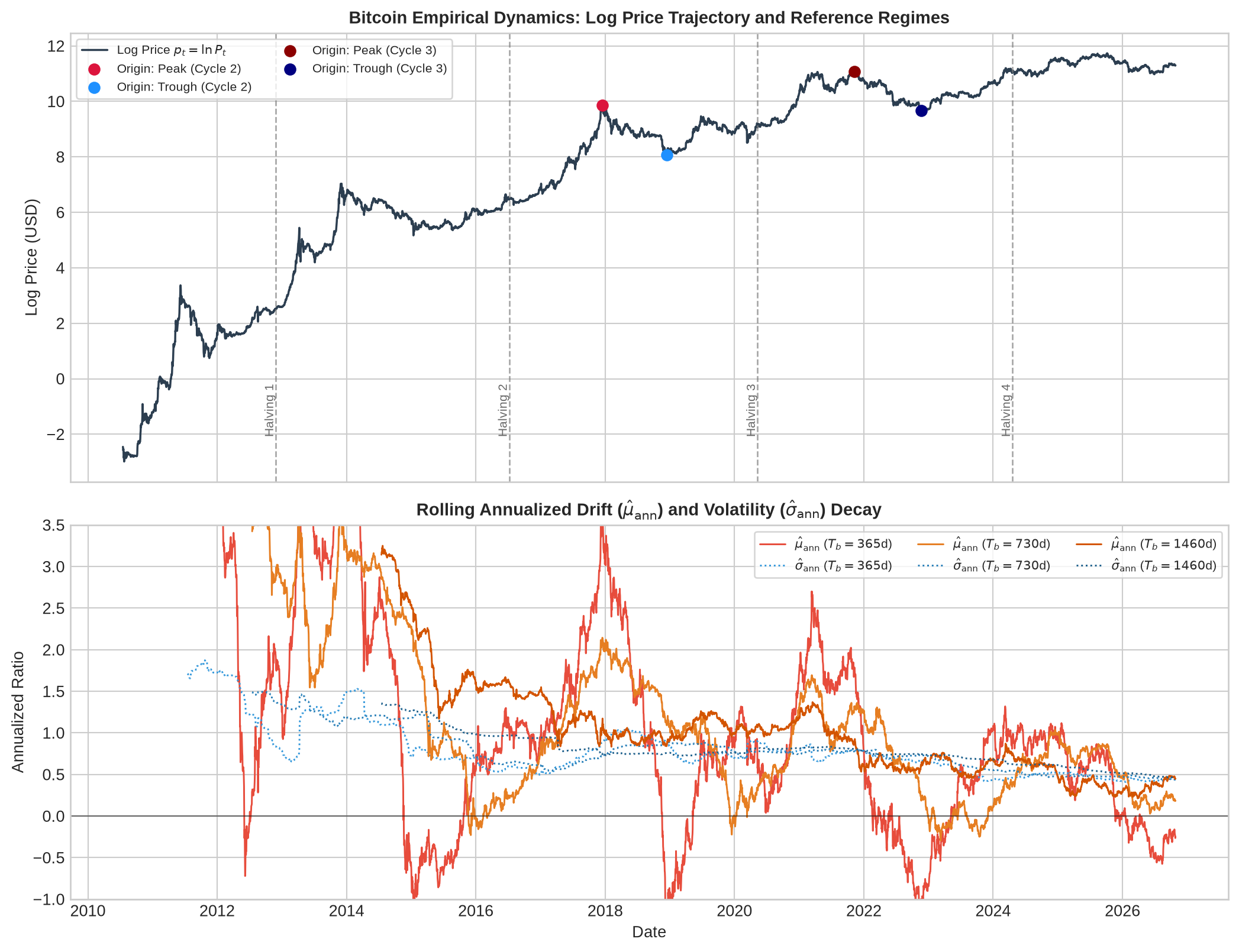
비트코인 로그 가격 궤적과 역사적 기준점, 그리고 롤링 연율화 모수의 비정상성 추이
           Regime  Obs Ann Drift Ann Vol  Skew Kurtosis JB p-val ADF p (p_t) ADF p (r_t)
      All History 5945   123.75%  88.66% -0.75    21.87  0.0e+00       0.064     8.2e-25
  Cycle 1 (Early)  864   310.11% 141.60% -0.20     8.85  0.0e+00       0.832     1.7e-19
          Cycle 2 1320   157.91%  97.78% -1.76    29.25  0.0e+00       0.275     1.8e-17
          Cycle 3 1403    99.96%  81.72% -0.94    12.98  0.0e+00       0.877     0.0e+00
          Cycle 4 1441    70.14%  62.09% -0.21     3.38 3.1e-152       0.754     0.0e+00
Cycle 5 (Current)  921    19.37%  44.69%  0.22     3.60 3.0e-110       0.737     0.0e+00

시계열 분석 결과는 비트코인 수익률 과정에 시간에 대해 일정한 모수를 가정하는 약정상성(Weak Stationarity) 전제가 기각됨을 실증한다.

초기 관측 구간인 Cycle 1에서 연율화 기대 수익률(\(\hat{\mu}_{\text{ann}}\))은 310.11%, 연율화 변동성(\(\hat{\sigma}_{\text{ann}}\))은 141.60%에 달했다. 시장 규모 확대와 제도권 유동성 편입이 진행되면서 Cycle 2(157.91%), Cycle 3(99.96%), Cycle 4(70.14%)를 거쳐 현재 Cycle 5에서는 연율화 드리프트가 19.37%로 축소되었다. 연율화 변동성 또한 동일 기간 141.60%에서 44.69% 수준으로 단조 감소하여, 수익률의 1차 및 2차 적률(Moment)이 시간 경과에 따라 하향 안정화되는 구조적 비정상성(Non-stationarity)을 드러낸다.

일간 로그 수익률(\(r_t\))의 경험적 분포는 강한 비정규성과 두터운 꼬리(Heavy Tails)를 갖는다. 전 기간 표본의 초과 첨도(Excess Kurtosis)는 21.87이며, Cycle 2 구간에서는 29.25까지 치솟는다. 자크-베라(Jarque-Bera) 정규성 검정의 유의확률(\(p\)-value)은 전 구간에서 \(10^{-100}\) 미만으로 산출되어 가우시안(Gaussian) 분포 가정이 유의수준 1% 미만에서 기각된다.

상수항과 선형 추세를 포함한 아우구멘티드 디키-풀러(ADF, Augmented Dickey-Fuller) 단위근 검정 결과, 수준 변수인 로그 가격 \(p_t\)의 유의확률(ADF p (p_t))은 전 기간 0.064 및 개별 사이클 0.275~0.877로 나타나 5% 유의수준에서 단위근 귀무가설을 기각하지 못하는 비정상 시계열(\(I(1)\))로 판별된다. 반면 1차 차분된 일간 로그 수익률 \(r_t\)는 전 구간에서 유의확률 \(10^{-16}\) 미만(ADF p (r_t))으로 단위근이 기각된다. 다만 차분 시계열이 단위근을 갖지 않더라도 평균 성장률 자체가 310.11%에서 19.37%로 감쇠하므로, 과거 전 기간 평균 드리프트(123.75%)를 고정 상수로 외삽하는 모형은 장기 지평에서 체계적인 상방 편향을 유발한다.


Models & Results

Structural Limitations of Historical Projections

과거 시계열 표본만을 외삽하여 장기 가격 경로를 추정하는 관행은 네 가지 구조적 왜곡(Structural Distortion)에 노출된다.

  • 시계열 표본 선택 및 생존 편향(Sample Selection and Survivorship Bias): 비트코인의 과거 16년 시계열은 생존 편향을 내포한다. 수많은 초기 대안 디지털 자산이 소멸하는 동안, 2010년대 글로벌 저금리와 유동성 확장기에 맞물려 생존한 단일 자산의 사후적 우상향 궤적만 표본으로 채택되었다. 거시 유동성 팽창이라는 외생적 조건이 자산 고유의 내재 성장률(Intrinsic Drift)로 치환되는 식별 오류(Identification Failure)가 발생한다.
  • 약정상성 가정의 붕괴(Failure of Weak Stationarity): 수익률 시계열의 기대값(\(\mu\))과 분산(\(\sigma^2\))이 시간 축에 대해 불변한다는 약정상성 가정이 성립하지 않는다. 시가총액 팽창, 기관 중심의 시장 미시구조(Market Microstructure) 재편, 파생상품 시장 성숙에 따라 기대 수익률과 변동성은 추세적으로 감쇠한다. 초기 급등기 표본의 \(\hat{\mu}\)를 장기 미래 지평(\(T_f\))에 지수 복리로 투사하면 기하급수적 상방 발산 오류(Explosive Divergence Bias)가 뒤따른다.
  • 구조적 체제 전환 미반영(Unaccounted Regime Shifts): 리테일 현물 중심 장세에서 기관 현물 ETF 및 옵션 딜러의 감마 헤징(Gamma Hedging)이 지배하는 장세로 전환되면서 데이터 생성 프로세스(Data Generating Process, DGP) 자체가 변모했다. 과거 체제에서 추출한 고정 모수는 변환된 시장 동학을 대표하지 못한다.
  • 팻 테일 및 미관측 외생 충격의 누락(Fat Tails and Unobserved Tail Risks): 정규분포 기반 확산 모형은 유동성 경색이나 연쇄 청산 같은 팻 테일(Fat-tail) 사건의 발생 확률을 과소평가한다. 비모수 재표본 추출(Non-parametric Resampling) 역시 과거 표본 공간 내부에 존재하지 않았던 새로운 외생적 충격(프로토콜 취약점, 거시적 규제 차단 등)에 대해서는 발생 확률을 0으로 할당하는 한계를 지닌다.

Experimental Design and Evaluation Metrics

모형 간 예측 안정성과 관측 창 의존도를 정량 비교하기 위해 아래 하이퍼파라미터 그리드(Hyperparameter Grid) 위에서 시뮬레이션을 수행한다.

Hyperparameter Symbol Test Values
Lookback Window \(T_b\) 365일 (1년), 730일 (2년), 1460일 (4년), All-history
Lookforward Horizon \(T_f\) 365일 (1년), 1460일 (4년; Cycle 3 Trough는 관측 가능한 1436일)
Reference Origin \(T_{\text{origin}}\) 2017-12-17 (고점), 2018-12-15 (저점), 2021-11-10 (고점), 2022-11-21 (저점)
Halving Cycle Period \(T_{\text{half\_life}}\) 1400일, 1460일, 1500일
Block Length (MBB) \(L\) 10일, 30일, 60일, 90일
Cycle Damping Factor \(\gamma\) 0.0 (미감쇠), 0.25 (중간 감쇠), 0.50 (강한 감쇠)
Monte Carlo Paths \(M\) 10,000

각 시나리오 조합별로 사후 실현 가격(Realized Price) \(P_{T_{\text{origin}} + k}\)와 \(M = 10,000\)개 시뮬레이션 경로 분포 간의 괴리를 두 가지 척도로 측정한다.

  1. 중앙값 예측 편향(Median Forecast Bias, \(\text{Bias}_{T_f}\)): 시뮬레이션 만기 분포의 중앙값과 실제 실현 가격 간의 상대 오차율을 산출하여 상방·하방 편향의 방향과 크기를 측정한다.

\[\text{Bias}_{T_f} = \frac{\text{Median}\left(P_{T_{\text{origin}} + T_f}^{(m)}\right) - P_{T_{\text{origin}} + T_f}}{P_{T_{\text{origin}} + T_f}}\]

  1. 경험적 신뢰구간 포괄률(Empirical Coverage Probability, \(\text{Coverage}_{90\%}\)): 예측 지평 \(k \in \{1, \dots, T_f\}\) 동안 실제 실현 가격 \(P_{T_{\text{origin}} + k}\)가 시뮬레이션 경로의 90% 예측 구간(\([q_{0.05, k}, \, q_{0.95, k}]\)) 내부에 머문 거래일 비율을 계산하여 불확실성 정량화의 적정성을 평가한다.

\[\text{Coverage}_{90\%} = \frac{1}{T_f} \sum_{k=1}^{T_f} \mathbb{I}\left( q_{0.05, k} \le P_{T_{\text{origin}} + k} \le q_{0.95, k} \right)\]

Code
import numpy as np
import pandas as pd

# 1. 시뮬레이션 하이퍼파라미터 상수 및 그리드 설정
ORIGINS = {
    "Cycle 2 Peak": pd.Timestamp("2017-12-17"),
    "Cycle 2 Trough": pd.Timestamp("2018-12-15"),
    "Cycle 3 Peak": pd.Timestamp("2021-11-10"),
    "Cycle 3 Trough": pd.Timestamp("2022-11-21")
}

T_B_LIST = [365, 730, 1460, "All"]
T_F_LIST = [365, 1460]
M_PATHS = 10000
RANDOM_SEED = 42

# 2. 표본 분할(In-sample 및 Out-of-sample) 슬라이싱 헬퍼 함수
def get_insample_data(data: pd.DataFrame, origin: pd.Timestamp, tb):
    """기준 시점(T_origin) 및 관측 창(T_b)에 해당하는 과거 시계열 추출"""
    sub = data[data["date"] <= origin].copy()
    if tb != "All":
        sub = sub.iloc[-int(tb):]
    return sub

def get_outsample_realized(data: pd.DataFrame, origin: pd.Timestamp, tf: int):
    """기준 시점 이후 실제 실현 가격(Realized Price, k = 1, ..., T_f) 궤적 추출"""
    sub = data[data["date"] > origin].head(tf).copy()
    return sub

# 3. 평가 지표 산출 헬퍼 함수
def compute_median_bias(sim_terminal_prices: np.ndarray, realized_price: float) -> float:
    """중앙값 예측 편향 (Bias_{T_f}) 산출"""
    median_val = np.median(sim_terminal_prices)
    return float((median_val - realized_price) / realized_price)

def compute_coverage_prob(sim_paths: np.ndarray, realized_prices: np.ndarray) -> float:
    """90% 신뢰구간 경험적 포괄률 (Coverage_{90%}) 산출 (k = 1, ..., T_f 정렬)"""
    steps = min(sim_paths.shape[1] - 1, len(realized_prices))
    q05, q95 = np.percentile(sim_paths[:, 1 : steps + 1], [5, 95], axis=0)
    realized = realized_prices[:steps]
    covered = (realized >= q05) & (realized <= q95)
    return float(np.mean(covered))

# 기준 시점별 실현 가격 및 표본 크기 검증 출력
verification_rows = []
for name, orig in ORIGINS.items():
    in_s = get_insample_data(df, orig, 365)
    out_1y = get_outsample_realized(df, orig, 365)
    out_4y = get_outsample_realized(df, orig, 1460)
    p0 = in_s.iloc[-1]["PriceUSD"]
    p_1y = out_1y.iloc[-1]["PriceUSD"]
    p_4y = out_4y.iloc[-1]["PriceUSD"]
    days_4y = len(out_4y)
    
    verification_rows.append({
        "Regime": name,
        "Cut-off Date": orig.strftime("%Y-%m-%d"),
        "P_0 (USD)": f"${p0:,.1f}",
        "Realized 1Y (P_365)": f"${p_1y:,.1f}",
        "Realized 4Y* (P_Tf)": f"${p_4y:,.1f} ({days_4y}d)"
    })

grid_status_df = pd.DataFrame(verification_rows)
print(grid_status_df.to_string(index=False))
        Regime Cut-off Date P_0 (USD) Realized 1Y (P_365) Realized 4Y* (P_Tf)
  Cycle 2 Peak   2017-12-17 $19,250.5            $3,499.2   $47,663.5 (1460d)
Cycle 2 Trough   2018-12-15  $3,185.1            $7,111.3   $17,809.7 (1460d)
  Cycle 3 Peak   2021-11-10 $64,756.1           $17,541.6  $104,685.5 (1460d)
Cycle 3 Trough   2022-11-21 $15,778.0           $36,035.0   $80,800.5 (1436d)

4개 기준 시점 중 Cycle 3 Trough(2022-11-21)는 표본 종료일(2026-10-27)까지 관측 가능한 미래 거래일이 1,436일(약 3.93년)이므로, 장기 지평 평가(4Y*) 시 해당 1,436일 구간의 실제 종가($80,800.5)를 기준으로 편향과 포괄률을 산출한다.


Parametric Method: Geometric Brownian Motion (GBM)

자산 가격 \(P_t\)가 연속 시간 기하 브라운 운동(Geometric Brownian Motion, GBM) 확률미분방정식(Stochastic Differential Equation, SDE)을 따른다고 가정한다.

\[dP_t = \mu_{\text{ann}} P_t dt + \sigma_{\text{ann}} P_t dW_t\]

Parameter Estimation and Discretization

기준 시점 \(T_{\text{origin}}\) 이전 관측 창 \([T_{\text{origin}} - T_b + 1, \, T_{\text{origin}}]\)에 속한 일간 로그 수익률 표본으로부터 일간 모수(\(\hat{\mu}_{\text{daily}}, \hat{\sigma}_{\text{daily}}\))와 이토 보조정리(Itô’s Lemma)가 반영된 연율화 모수(\(\hat{\mu}_{\text{ann}}, \hat{\sigma}_{\text{ann}}\))를 추정한다.

\[\hat{\mu}_{\text{daily}} = \frac{1}{T_b} \sum_{t=T_{\text{origin}}-T_b+1}^{T_{\text{origin}}} r_t, \quad \hat{\sigma}_{\text{daily}}^2 = \frac{1}{T_b - 1} \sum_{t=T_{\text{origin}}-T_b+1}^{T_{\text{origin}}} (r_t - \hat{\mu}_{\text{daily}})^2\]

\[\hat{\sigma}_{\text{ann}} = \frac{\hat{\sigma}_{\text{daily}}}{\sqrt{\Delta t}}, \quad \hat{\mu}_{\text{ann}} = \frac{\hat{\mu}_{\text{daily}}}{\Delta t} + \frac{1}{2}\hat{\sigma}_{\text{ann}}^2\]

오일러-마루야마 이산화(Euler-Maruyama Discretization)를 적용한 예측 단계 \(k \in \{1, 2, \dots, T_f\}\)에서의 \(m\)번째 시뮬레이션 경로 전개식은 다음과 같다.

\[P_{T_{\text{origin}} + k}^{(m)} = P_{T_{\text{origin}} + k - 1}^{(m)} \exp\left( \left( \hat{\mu}_{\text{ann}} - \frac{1}{2}\hat{\sigma}_{\text{ann}}^2 \right)\Delta t + \hat{\sigma}_{\text{ann}} \sqrt{\Delta t} Z_k^{(m)} \right), \quad Z_k^{(m)} \sim \text{i.i.d. } \mathcal{N}(0, 1)\]

초기 가격은 \(P_{T_{\text{origin}}}^{(m)} = P_{T_{\text{origin}}}\)으로 고정한다.

Code
import matplotlib.pyplot as plt

# 1. GBM 시뮬레이션 벡터화 함수 정의
def simulate_gbm_paths(sub_series: pd.Series, p0: float, tf: int, m_paths: int = 10000, seed: int = 42):
    """표본 로그 수익률로부터 연율화 모수를 추정하고 오일러-마루야마 GBM 경로 생성"""
    r = sub_series.dropna().values
    d_mu = np.mean(r)
    d_vol = np.std(r, ddof=1)
    sig_ann = d_vol / np.sqrt(dt)
    mu_ann = (d_mu / dt) + 0.5 * (sig_ann ** 2)
    
    np.random.seed(seed)
    drift = (mu_ann - 0.5 * sig_ann**2) * dt
    diffusion = sig_ann * np.sqrt(dt) * np.random.randn(m_paths, tf)
    increments = drift + diffusion
    log_paths = np.hstack([np.zeros((m_paths, 1)), np.cumsum(increments, axis=1)])
    paths = p0 * np.exp(log_paths)
    return paths, mu_ann, sig_ann

# 2. 4개 체제 x 4개 관측 창 모수 추정 및 성과 집계 (시뮬레이션 결과 캐싱)
gbm_summary_rows = []
gbm_cache = {}
tb_display_list = [365, 730, 1460, "All"]

for origin_name, origin_date in ORIGINS.items():
    realized_df = get_outsample_realized(df, origin_date, 1460)
    tf_len = len(realized_df)
    p_real_1y = realized_df.iloc[364]["PriceUSD"]
    p_real_end = realized_df.iloc[-1]["PriceUSD"]
    
    for tb in tb_display_list:
        insample_df = get_insample_data(df, origin_date, tb)
        p0 = insample_df.iloc[-1]["PriceUSD"]
        paths, mu_ann, sig_ann = simulate_gbm_paths(insample_df["r_t"], p0, tf_len, M_PATHS, RANDOM_SEED)
        gbm_cache[(origin_name, tb)] = paths
        
        bias_1y = compute_median_bias(paths[:, 365], p_real_1y)
        cov_1y = compute_coverage_prob(paths[:, :366], realized_df.iloc[:365]["PriceUSD"].values)
        bias_4y = compute_median_bias(paths[:, -1], p_real_end)
        cov_4y = compute_coverage_prob(paths, realized_df["PriceUSD"].values)
        
        gbm_summary_rows.append({
            "Origin": origin_name,
            "T_b": str(tb),
            "mu_ann": f"{mu_ann:.1%}",
            "sig_ann": f"{sig_ann:.1%}",
            "Med 1Y": f"${np.median(paths[:, 365]):,.0f}",
            "Bias (1Y)": f"{bias_1y:+.1%}",
            "Cov (1Y)": f"{cov_1y:.1%}",
            "Med 4Y*": f"${np.median(paths[:, -1]):,.0f}",
            "Bias (4Y*)": f"{bias_4y:+.1%}",
            "Cov (4Y*)": f"{cov_4y:.1%}"
        })

gbm_results_df = pd.DataFrame(gbm_summary_rows)
print(gbm_results_df.to_string(index=False))

# 3. 2x2 서브플롯 팬 차트(Fan Chart) 시각화
fig, axes = plt.subplots(2, 2, figsize=(14, 10), sharey=False)
palette = {"365": "#e74c3c", "1460": "#3498db", "All": "#2ecc71"}

for ax, (origin_name, origin_date) in zip(axes.flatten(), ORIGINS.items()):
    realized_df = get_outsample_realized(df, origin_date, 1460)
    t_days = np.arange(len(realized_df) + 1)
    
    in_last = get_insample_data(df, origin_date, 1).iloc[-1]["PriceUSD"]
    p_real_series = np.array([in_last] + realized_df["PriceUSD"].tolist())
    ax.plot(t_days, p_real_series, color="black", lw=2.0, zorder=6, label="Realized Price")
    
    for tb in [365, 1460, "All"]:
        paths = gbm_cache[(origin_name, tb)]
        q05, q50, q95 = np.percentile(paths, [5, 50, 95], axis=0)
        
        c = palette[str(tb)]
        ax.plot(t_days, q50, color=c, lw=1.3, label=rf"Median ($T_b={tb}$)")
        ax.fill_between(t_days, q05, q95, color=c, alpha=0.15)
        
    ax.set_yscale("log")
    ax.set_title(f"Regime: {origin_name} ({origin_date.strftime('%Y-%m-%d')})", fontsize=11, fontweight="bold")
    ax.set_xlabel("Days Elapsed from Cut-off ($k$)", fontsize=9)
    ax.set_ylabel("Price in USD (Log Scale)", fontsize=9)
    ax.legend(loc="upper left" if "Trough" in origin_name else "lower left", fontsize=7.5, frameon=True)

plt.tight_layout()
plt.show()
        Origin  T_b  mu_ann sig_ann   Med 1Y Bias (1Y) Cov (1Y)        Med 4Y*   Bias (4Y*) Cov (4Y*)
  Cycle 2 Peak  365  359.2%   89.2% $476,038 +13504.4%     1.1% $6,716,025,632 +14090409.5%      0.3%
  Cycle 2 Peak  730  212.7%   72.6% $125,548  +3487.9%     1.1%    $32,914,670    +68956.4%      0.3%
  Cycle 2 Peak 1460  117.3%   73.9%  $47,906  +1269.1%     1.1%       $697,063     +1362.5%     10.3%
  Cycle 2 Peak  All  227.1%  110.5% $103,044  +2844.8%     4.7%    $14,502,206    +30326.2%      1.2%
Cycle 2 Trough  365 -134.8%   85.7%     $581    -91.8%    26.6%             $3      -100.0%      6.6%
Cycle 2 Trough  730  109.3%   88.0%   $6,543     -8.0%    99.2%        $52,972      +197.4%     99.8%
Cycle 2 Trough 1460   85.4%   75.7%   $5,688    -20.0%    93.4%        $30,544       +71.5%     98.4%
Cycle 2 Trough  All  183.3%  108.0%  $11,311    +59.1%    99.7%       $465,779     +2515.3%     99.9%
  Cycle 3 Peak  365  175.3%   78.9% $277,191  +1480.2%     8.2%    $20,446,561    +19431.4%      2.1%
  Cycle 3 Peak  730  130.6%   77.8% $178,737   +918.9%    18.1%     $3,537,707     +3279.4%      4.5%
  Cycle 3 Peak 1460   90.6%   80.6% $117,230   +568.3%    44.4%       $653,246      +524.0%     64.0%
  Cycle 3 Peak  All  170.4%  100.8% $217,433  +1139.5%    44.4%     $7,610,137     +7169.5%     11.1%
Cycle 3 Trough  365 -109.3%   67.2%   $4,256    -88.2%    14.5%            $87       -99.9%      3.7%
Cycle 3 Trough  730   18.6%   73.6%  $14,638    -59.4%   100.0%        $11,149       -86.2%     65.4%
Cycle 3 Trough 1460   60.4%   74.7%  $22,058    -38.8%   100.0%        $55,919       -30.8%    100.0%
Cycle 3 Trough  All  146.7%   98.5%  $42,665    +18.4%   100.0%       $736,962      +812.1%    100.0%

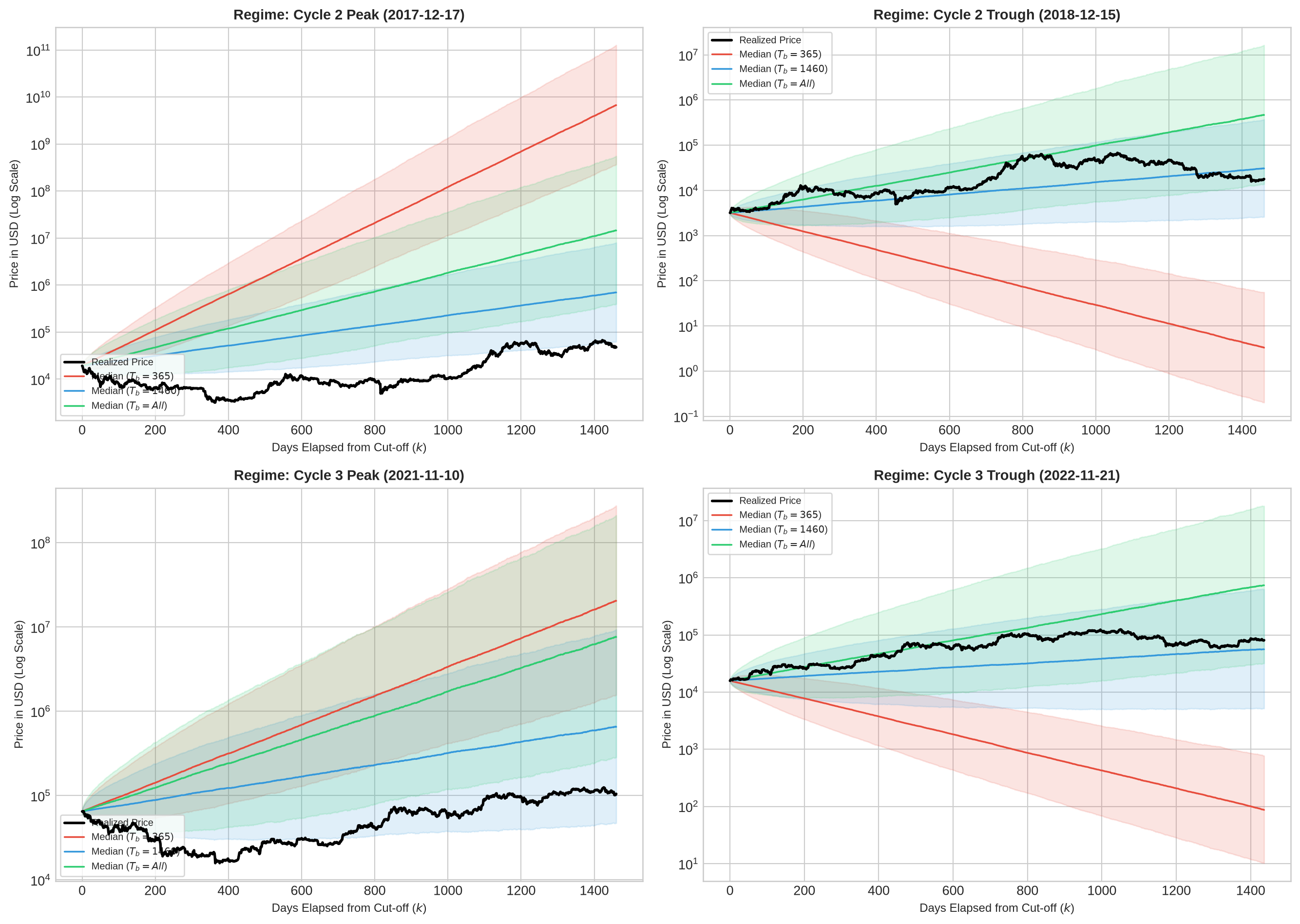
기하 브라운 운동(GBM) 시뮬레이션 경로: 관측 창(T_b) 및 기준 국면(T_origin)별 경로 발산과 실제 실현 가격 비교

기하 브라운 운동(GBM) 시뮬레이션 결과는 관측 창(\(T_b\))과 기준 시점(\(T_{\text{origin}}\))의 조합에 따라 만기 예측 분포가 수백 배에서 수만 배까지 발산하는 모수 불안정성(Parametric Instability)을 보여준다.

강세장 정점인 Cycle 2 Peak(2017-12-17, \(P_0 = \$19,250.5\))에서 1년 관측 창(\(T_b=365\))을 적용하면 추정 연율화 드리프트(\(\hat{\mu}_{\text{ann}}\))가 359.2%, 변동성(\(\hat{\sigma}_{\text{ann}}\))이 89.2%에 달한다. 높은 양(+)의 표본 드리프트가 연속 복리로 증폭되면서 1년 후 예측 중앙값은 47만 6,038달러로 산출되어 실제 실현 가격(3,499.2달러) 대비 중앙값 예측 편향(\(\text{Bias}_{365}\))이 +13,504.4%에 이른다. 1년 예측 구간 포괄률(\(\text{Coverage}_{365}\))은 1.1%에 불과하며, 4년 지평(\(T_f=1460\))에서는 예측 중앙값이 약 67억 1,603만 달러(\(\text{Bias}_{1460} = +14,090,409.5\%\))로 폭증하여 경제적 의미를 상실한다.

반대로 약세장 저점인 Cycle 2 Trough(2018-12-15, \(P_0 = \$3,185.1\))에서 \(T_b=365\)를 적용하면 직전 1년간의 급락 장세가 그대로 반영되어 연율화 드리프트가 -134.8%로 추정된다. 음(-)의 드리프트 외삽에 의해 1년 후 예측 중앙값은 581달러로 하락하여 실제 실현 가격(7,111.3달러) 대비 -91.8%의 하방 편향을 기록했고, 4년 후 예측 중앙값은 3달러(\(\text{Bias}_{1460} = -100.0\%\), 포괄률 6.6%)로 수렴하여 사후적인 반등 국면(1만 7,809.7달러)을 놓쳤다. Cycle 3 Trough(2022-11-21)의 \(T_b=365\) 조건에서도 동일하게 \(\hat{\mu}_{\text{ann}} = -109.3\%\)가 추정되어 장기 중앙값이 87달러(-99.9% 편향)로 추락했다.

관측 창을 4년(\(T_b=1460\), 반감기 1주기)으로 확장하면 단기 급등락에 의한 왜곡은 완화되나, 직전 사이클의 높은 평균 성장률이 여전히 이월되어 Cycle 2 Peak와 Cycle 3 Peak의 4년 예측 편향이 각각 +1,362.5% 및 +524.0%로 나타난다. 전 기간(\(T_b=\text{All}\)) 표본을 사용할 경우 2010~2013년 초기 급등기 드리프트가 합산되면서 Cycle 3 Peak 기준 4년 예측 중앙값이 761만 달러(\(\text{Bias}_{1460} = +7,169.5\%\))로 재차 발산한다. 고정 모수 확산 모형에서는 표본 길이를 단순히 늘리는 것만으로는 성장률 체감에 따른 상방 편향을 제거할 수 없다.


Non-Parametric Method: Moving Block Bootstrapping (MBB)

정규분포 가정을 제거하고 경험적 수익률 분포(Empirical Return Distribution)의 비대칭성과 두터운 꼬리(Heavy Tails)를 보존하기 위해 비모수 부트스트랩을 도입한다. 단순 독립동일분포(i.i.d.) 복원 추출은 금융 시계열 고유의 변동성 군집(Volatility Clustering)과 단기 자기상관(Autocorrelation)을 파괴하므로, 연속된 \(L\)일 길이의 블록 단위로 복원 추출하는 이동 블록 부트스트랩(Moving Block Bootstrap, MBB)을 적용한다.

Block Pool Construction and Path Generation

  1. 중첩 블록 풀(Overlapping Block Pool) 구성: 관측 창 내부의 로그 수익률 벡터 \((r_{T_{\text{origin}}-T_b+1}, \dots, r_{T_{\text{origin}}})\)에서 길이 \(L\)인 \(N_B = T_b - L + 1\)개의 연속 중첩 블록 \(B_j\)를 추출한다.

\[B_j = (r_j, r_{j+1}, \dots, r_{j+L-1}), \quad j \in \{T_{\text{origin}}-T_b+1, \dots, T_{\text{origin}}-L+1\}\]

  1. 블록 복원 추출 및 접합: 예측 지평 \(T_f\)를 덮기 위해 \(K = \lceil T_f / L \rceil\)개의 블록을 균등 확률로 무작위 복원 추출(Sampling with Replacement)하여 순서대로 연결한 뒤, 앞선 \(T_f\)개 원소를 절단하여 합성 수익률 경로 \(r^{*(m)} = (r_1^{*(m)}, r_2^{*(m)}, \dots, r_{T_f}^{*(m)})\)를 구성한다.
  2. 시뮬레이션 가격 경로 생성:

\[P_{T_{\text{origin}} + k}^{(m)} = P_{T_{\text{origin}}} \exp\left( \sum_{i=1}^{k} r_i^{*(m)} \right), \quad k \in \{1, \dots, T_f\}\]

Code
# 1. MBB 시뮬레이션 벡터화 함수 정의
def simulate_mbb_paths(sub_series: pd.Series, p0: float, block_len: int, tf: int, m_paths: int = 10000, seed: int = 42):
    """과거 관측 창의 로그 수익률 벡터로부터 중첩 블록 풀을 구성하고 MBB 가격 경로 생성"""
    r = sub_series.dropna().values
    n_b = len(r) - block_len + 1
    blocks = np.array([r[i : i + block_len] for i in range(n_b)])
    k_blocks = int(np.ceil(tf / block_len))
    
    np.random.seed(seed)
    block_indices = np.random.randint(0, n_b, size=(m_paths, k_blocks))
    sampled_returns = blocks[block_indices].reshape(m_paths, -1)[:, :tf]
    log_paths = np.hstack([np.zeros((m_paths, 1)), np.cumsum(sampled_returns, axis=1)])
    return p0 * np.exp(log_paths)

# 2. 반감기 1주기 관측 창(T_b = 1460) 기준 블록 길이(L in {10, 30, 60, 90}) 민감도 및 GBM 대조
mbb_summary_rows = []
block_lengths = [10, 30, 60, 90]
mbb_cache = {}

for peak_name in ["Cycle 2 Peak", "Cycle 3 Peak"]:
    orig_date = ORIGINS[peak_name]
    in_1460 = get_insample_data(df, orig_date, 1460)
    p0_val = in_1460.iloc[-1]["PriceUSD"]
    real_df = get_outsample_realized(df, orig_date, 1460)
    p_real_4y = real_df.iloc[-1]["PriceUSD"]
    
    # GBM 벤치마크 (캐시 재사용)
    gbm_p = gbm_cache[(peak_name, 1460)]
    g_q05, g_q50, g_q95 = np.percentile(gbm_p[:, -1], [5, 50, 95])
    g_cov = compute_coverage_prob(gbm_p, real_df["PriceUSD"].values)
    g_bias = compute_median_bias(gbm_p[:, -1], p_real_4y)
    
    mbb_summary_rows.append({
        "Origin": peak_name,
        "Model / Block (L)": "GBM (Tb=1460)",
        "4Y 5th Pct": f"${g_q05:,.0f}",
        "4Y Median": f"${g_q50:,.0f}",
        "4Y 95th Pct": f"${g_q95:,.0f}",
        "Bias (4Y)": f"{g_bias:+.1%}",
        "Coverage (4Y)": f"{g_cov:.1%}"
    })
    
    for L in block_lengths:
        paths_mbb = simulate_mbb_paths(in_1460["r_t"], p0_val, L, 1460, M_PATHS, RANDOM_SEED)
        mbb_cache[(peak_name, L)] = paths_mbb
        
        q05, q50, q95 = np.percentile(paths_mbb[:, -1], [5, 50, 95])
        cov = compute_coverage_prob(paths_mbb, real_df["PriceUSD"].values)
        bias = compute_median_bias(paths_mbb[:, -1], p_real_4y)
        
        mbb_summary_rows.append({
            "Origin": peak_name,
            "Model / Block (L)": f"MBB (L={L}d)",
            "4Y 5th Pct": f"${q05:,.0f}",
            "4Y Median": f"${q50:,.0f}",
            "4Y 95th Pct": f"${q95:,.0f}",
            "Bias (4Y)": f"{bias:+.1%}",
            "Coverage (4Y)": f"{cov:.1%}"
        })

mbb_table_df = pd.DataFrame(mbb_summary_rows)
print(mbb_table_df.to_string(index=False))

# 3. GBM vs MBB 비교 시각화 (Cycle 3 Peak 기준 팬 차트 및 블록 길이별 분위수 분포)
fig, (ax_left, ax_right) = plt.subplots(1, 2, figsize=(14, 5.5))

target_peak = "Cycle 3 Peak"
orig_dt = ORIGINS[target_peak]
in_target = get_insample_data(df, orig_dt, 1460)
p0_t = in_target.iloc[-1]["PriceUSD"]
real_t = get_outsample_realized(df, orig_dt, 1460)
p_real_t4y = real_t.iloc[-1]["PriceUSD"]
t_eval = np.arange(1461)
p_real_eval = np.array([p0_t] + real_t["PriceUSD"].tolist())

# Panel 1: Cycle 3 Peak - GBM vs MBB (L=30, Tb=1460)
ax_left.plot(t_eval, p_real_eval, color="black", lw=2.0, zorder=6, label="Realized Price")

gbm_ref = gbm_cache[(target_peak, 1460)]
g05, g50, g95 = np.percentile(gbm_ref, [5, 50, 95], axis=0)
ax_left.plot(t_eval, g50, color="#e74c3c", lw=1.5, label="GBM Median (Tb=1460)")
ax_left.fill_between(t_eval, g05, g95, color="#e74c3c", alpha=0.15, label="GBM 90% CI")

mbb_l30 = mbb_cache[(target_peak, 30)]
m05, m50, m95 = np.percentile(mbb_l30, [5, 50, 95], axis=0)
ax_left.plot(t_eval, m50, color="#3498db", lw=1.5, linestyle="--", label="MBB (L=30) Median")
ax_left.fill_between(t_eval, m05, m95, color="#3498db", alpha=0.2, label="MBB (L=30) 90% CI")

ax_left.set_yscale("log")
ax_left.set_title("Cycle 3 Peak: GBM vs MBB (L=30d, Tb=1460d)", fontsize=11, fontweight="bold")
ax_left.set_xlabel("Days Elapsed ($k$)", fontsize=9)
ax_left.set_ylabel("Price in USD (Log Scale)", fontsize=9)
ax_left.legend(loc="upper left", fontsize=8, frameon=True)

# Panel 2: 블록 길이(L)별 4년 만기 가격 분위수 및 실제 실현 가격 비교 (Cycle 3 Peak)
l_labels = ["GBM"] + [f"MBB (L={l})" for l in block_lengths]
term_arrays = [gbm_ref[:, -1]] + [mbb_cache[(target_peak, l)][:, -1] for l in block_lengths]
q05_vals = [np.percentile(p, 5) for p in term_arrays]
q50_vals = [np.percentile(p, 50) for p in term_arrays]
q95_vals = [np.percentile(p, 95) for p in term_arrays]

x_idx = np.arange(len(l_labels))
ax_right.plot(x_idx, q50_vals, marker="o", color="#2c3e50", lw=1.5, label="Terminal Median")
ax_right.vlines(x_idx, q05_vals, q95_vals, color="#7f8c8d", lw=3.0, alpha=0.7, label="90% Forecast Band [5%, 95%]")
ax_right.axhline(p_real_t4y, color="black", linestyle="--", lw=1.2, label=f"Realized 4Y Price (${p_real_t4y:,.0f})")

ax_right.set_yscale("log")
ax_right.set_xticks(x_idx)
ax_right.set_xticklabels(l_labels, rotation=20, ha="right", fontsize=8.5)
ax_right.set_title("Cycle 3 Peak: 4-Year Terminal Dispersion Across Block Lengths", fontsize=11, fontweight="bold")
ax_right.set_ylabel("Terminal Price in USD (Log Scale)", fontsize=9)
ax_right.legend(loc="upper right", fontsize=8, frameon=True)

plt.tight_layout()
plt.show()
      Origin Model / Block (L) 4Y 5th Pct 4Y Median 4Y 95th Pct Bias (4Y) Coverage (4Y)
Cycle 2 Peak     GBM (Tb=1460)    $62,501  $697,063  $7,982,138  +1362.5%         10.3%
Cycle 2 Peak       MBB (L=10d)    $46,096  $516,199  $5,817,915   +983.0%         20.8%
Cycle 2 Peak       MBB (L=30d)    $27,498  $305,952  $4,140,257   +541.9%         26.7%
Cycle 2 Peak       MBB (L=60d)    $19,753  $244,415  $3,441,091   +412.8%         30.3%
Cycle 2 Peak       MBB (L=90d)    $16,818  $219,189  $3,002,320   +359.9%         33.6%
Cycle 3 Peak     GBM (Tb=1460)    $47,081  $653,246  $9,328,379   +524.0%         64.0%
Cycle 3 Peak       MBB (L=10d)    $35,960  $579,815  $9,372,373   +453.9%         75.1%
Cycle 3 Peak       MBB (L=30d)    $22,882  $435,783  $7,876,889   +316.3%         81.5%
Cycle 3 Peak       MBB (L=60d)    $18,076  $307,041  $5,610,999   +193.3%         83.4%
Cycle 3 Peak       MBB (L=90d)    $16,578  $311,350  $6,657,957   +197.4%         84.1%

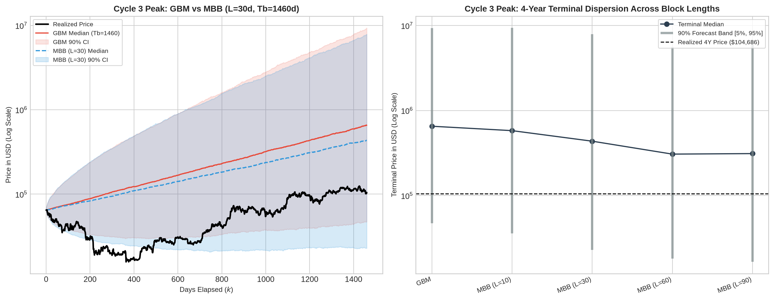
이동 블록 부트스트랩(MBB) 시뮬레이션: 4년 주기 관측 창(T_b=1460) 하에서 GBM 대비 꼬리 위험(Tail Risk) 보존 특성 및 블록 길이(L) 민감도

반감기 1주기 길이의 관측 창(\(T_b=1460\))에서 수행한 이동 블록 부트스트랩(MBB) 실험은 비모수 블록 추출이 하방 꼬리 위험(Downside Tail Risk) 포착력을 개선하는 과정과, 추세 비정상성을 제거하지 못할 때 남는 한계를 동시에 보여준다.

블록 길이(\(L\))를 10일에서 90일로 늘릴수록 중첩 블록 풀은 단기 일간 노이즈가 아니라 중기 연속 급락 장세(Drawdown Clusters)와 변동성 군집을 보존하여 추출한다. Cycle 2 Peak(\(T_b=1460\), 4년 후 실현 가격 4만 7,663달러)에서 가우시안 대칭 확산을 가정한 GBM은 4년 만기 하방 5% 분위수를 6만 2,501달러로 산출하여, 실현 가격조차 하방 5% 경계 아래에 놓이는 과신(포괄률 10.3%)을 범했다. 반면 MBB는 블록 길이 \(L\)을 10일, 30일, 60일, 90일로 확장함에 따라 4년 만기 하방 5% 분위수를 각각 4만 6,096달러, 2만 7,498달러, 1만 9,753달러, 1만 6,818달러로 낮추었으며, 4년 예측 구간 포괄률도 GBM의 10.3%에서 33.6%(\(L=90\))로 3배 이상 높였다. Cycle 3 Peak(\(T_b=1460\))에서도 MBB(\(L=30\))의 4년 포괄률은 81.5%를 기록하여 GBM(64.0%) 대비 우위를 보였다.

비모수 부트스트랩 단독 사용의 구조적 한계 또한 수치로 확인된다. MBB는 관측 창(\(T_b\)) 내부의 수익률 블록을 동일 확률로 복원 추출하므로, 합성 경로의 기대 로그 성장률은 표본 관측 창의 산술 평균 수익률(\(\bar{r}_{T_b}\))에 구속된다. 직전 4년 사이클(Cycle 2 및 Cycle 3)의 평균 성장률이 후속 사이클보다 높았던 탓에, \(L=30\) 기준 MBB의 4년 만기 중앙값은 Cycle 2 Peak에서 30만 5,952달러(편향 +541.9%), Cycle 3 Peak에서 43만 5,783달러(편향 +316.3%)로 산출되어 상당한 상방 편향이 잔존했다. 비모수 재표본 추출이 유효하게 작동하려면 원계열에서 장기 성장률 체감 추세와 반감기 주기를 먼저 분리해야 한다.


Semi-Parametric Method: Trend and Halving Cycle Decomposition

장기 비정상성(성장률 체감)과 반감기 주기에 따른 순환 변동을 명시적으로 통제하기 위해, 로그 가격 시계열 \(p_t\)를 구조적 추세 성분(Structural Trend), 주기적 순환 성분(Cyclical Component), 정상적 확률 잔차(Stationary Residual)로 가법 분해(Additive Decomposition)한 뒤 잔차의 자기회귀 혁신항(Innovation)에 MBB를 결합하는 준모수 모형을 구축한다.

\[p_t = p_{\text{trend}}(t) + c(t) + \epsilon_t\]

Diminishing Growth Rate (Power-Law Trend)

자산 시가총액 확대와 시장 성숙에 따른 기대 성장률의 구조적 체감을 제네시스 블록 이후 경과 일수 \(t\)에 대한 거듭제곱 법칙(Power-Law Trend)으로 모형화한다.

\[p_{\text{trend}}(t) = a + b \ln(t)\]

모수 \((a, b)\)는 미래 정보 누수(Look-ahead Bias)를 차단하기 위해 기준 시점 이전 구간(\(t \le T_{\text{origin}}\))의 표본만으로 최소제곱법(OLS)을 통해 추정한다. 로그 시간 축에 대한 선형 함수이므로 시간 경과에 따른 순간 기대 성장률 \(\frac{dp_{\text{trend}}(t)}{dt} = \frac{b}{t}\)은 \(t\)가 커짐에 따라 \(1/t\)에 비례하여 감쇠한다.

Business Cycle (Halving-Induced Cyclicality)

반감기 주기 \(T_{\text{half\_life}}\)에 연동된 공급 충격 순환과 시장 성숙에 따른 진폭 축소(Amplitude Damping)를 감쇠 조화 진동자(Damped Harmonic Oscillator) 함수로 정식화한다.

\[c(t) = A_0 \cdot t^{-\gamma} \sin\left(\frac{2\pi t}{T_{\text{half\_life}}} + \phi\right) = t^{-\gamma} \left[ \beta_1 \sin\left(\frac{2\pi t}{T_{\text{half\_life}}}\right) + \beta_2 \cos\left(\frac{2\pi t}{T_{\text{half\_life}}}\right) \right]\]

여기서 \(A_0 = \sqrt{\beta_1^2 + \beta_2^2}\)는 초기 순환 진폭, \(\gamma \ge 0\)는 시간 경과에 따른 진폭 감쇠율(Damping Factor), \(\phi = \text{atan2}(\beta_2, \beta_1)\)는 반감기 시점 정렬을 위한 위상각(Phase Shift)이다. 삼각함수 덧셈정리를 통해 선형 회귀 행렬 \(X = [1, \, \ln t, \, t^{-\gamma}\sin(\omega t), \, t^{-\gamma}\cos(\omega t)]\)을 구성하면 주어진 \((\gamma, T_{\text{half\_life}})\) 하에서 전역 최적해 \((\hat{a}, \hat{b}, \hat{\beta}_1, \hat{\beta}_2)\)가 닫힌 형식(Closed-form OLS)으로 유일하게 결정된다.

Stationary Residual AR(1) Filtering and Path Synthesis

기준 시점 이전 관측 구간에서 추정된 추세와 순환 성분을 차감하여 구조적 잔차 시계열 \(\hat{\epsilon}_t\)를 분리한다.

\[\hat{\epsilon}_t = p_t - \left( \hat{p}_{\text{trend}}(t) + \hat{c}(t) \right)\]

분리된 잔차 \(\hat{\epsilon}_t\)는 평균이 0이고 단위근이 기각되는 정상 시계열(\(I(0)\))이다. 만일 정상 시계열인 \(\hat{\epsilon}_t\)의 1차 차분(\(\Delta \hat{\epsilon}_t\))을 블록 복원 추출하여 단순 누적합(\(\hat{\epsilon}_{T_{\text{origin}}} + \sum_{i=1}^k \Delta \epsilon_i^*\))으로 외삽하면 두 가지 계량경제학적 오류가 발생한다. 첫째, 강세장 고점의 양(+)의 거품 잔차(\(\hat{\epsilon}_{T_{\text{origin}}} > 0\))나 약세장 저점의 음(-)의 과매도 잔차(\(\hat{\epsilon}_{T_{\text{origin}}} < 0\))가 장기 평균(0)으로 평균회귀(Mean Reversion)하지 않고 영구 고정된다. 둘째, 블록 경계에서 장기 음(-)의 자기공분산이 절단되면서 누적 잔차의 분산이 예측 지평 \(k\)에 비례하여 무한 발산(\(\text{Var} \propto k\))하는 인위적 단위근(Random Walk) 현상이 주입된다.

평균회귀 동학과 잔차의 비정규 변동성 군집을 동시에 보존하기 위해, 기준 시점 이전 잔차 표본에서 1차 자기회귀 계수 \(\hat{\rho} \in (0, 1)\)와 중심화된 경험적 혁신항(Innovation) \(\hat{u}_t\)를 추출한다.

\[\hat{\epsilon}_t = \hat{\rho} \hat{\epsilon}_{t-1} + \hat{u}_t, \quad \hat{\rho} = \frac{\sum_{t=2}^{T_{\text{origin}}} \hat{\epsilon}_{t-1} \hat{\epsilon}_t}{\sum_{t=2}^{T_{\text{origin}}} \hat{\epsilon}_{t-1}^2}\]

혁신항 벡터 \((\hat{u}_2, \dots, \hat{u}_{T_{\text{origin}}})\)에 길이 \(L\)의 이동 블록 부트스트랩(MBB)을 적용하여 부트스트랩 혁신 경로 \(u_k^{*(m)}\)를 생성한 뒤, 초기 잔차 \(\hat{\epsilon}_{T_{\text{origin}}}\)로부터 자기회귀 필터링을 수행하여 예측 시점 \(T_{\text{origin}} + k\)의 잔차 경로 \(\epsilon_{T_{\text{origin}} + k}^{*(m)}\)와 시뮬레이션 가격 \(P_{T_{\text{origin}} + k}^{(m)}\)를 합성한다.

\[\epsilon_{T_{\text{origin}} + k}^{*(m)} = \hat{\rho}^k \hat{\epsilon}_{T_{\text{origin}}} + \sum_{i=1}^{k} \hat{\rho}^{k - i} u_i^{*(m)}\]

\[p_{T_{\text{origin}} + k}^{(m)} = \hat{p}_{\text{trend}}(T_{\text{origin}} + k) + \hat{c}(T_{\text{origin}} + k) + \epsilon_{T_{\text{origin}} + k}^{*(m)}, \quad P_{T_{\text{origin}} + k}^{(m)} = \exp\left( p_{T_{\text{origin}} + k}^{(m)} \right)\]

Code
# 1. 준모수 가법 분해 및 AR(1) 혁신항 추출 함수
def fit_semi_parametric(data_slice: pd.DataFrame, gamma: float = 0.25, t_half: float = 1460.0):
    """로그 가격을 거듭제곱 추세, 감쇠 조화 진동자, AR(1) 정상 잔차로 분해"""
    t = data_slice["t"].values
    p = data_slice["p_t"].values
    ln_t = np.log(t)
    omega = 2.0 * np.pi / t_half
    sin_term = (t ** -gamma) * np.sin(omega * t)
    cos_term = (t ** -gamma) * np.cos(omega * t)
    
    X = np.column_stack([np.ones_like(t), ln_t, sin_term, cos_term])
    beta, _, _, _ = np.linalg.lstsq(X, p, rcond=None)
    
    p_trend = beta[0] + beta[1] * ln_t
    c = beta[2] * sin_term + beta[3] * cos_term
    residual = p - (p_trend + c)
    
    # 잔차의 AR(1) 평균회귀 계수(rho) 및 혁신항(u_t) 추정
    res_lag = residual[:-1]
    res_curr = residual[1:]
    rho = float(np.clip(np.sum(res_lag * res_curr) / np.sum(res_lag ** 2), 0.0, 0.999))
    innovations = res_curr - rho * res_lag
    innovations = innovations - np.mean(innovations)
    return beta, p_trend, c, residual, rho, innovations

# 2. 준모수 경로 생성 함수 (외삽 추세 + 감쇠 사이클 + AR(1)-MBB 잔차 필터링)
def simulate_semi_parametric_paths(data_slice: pd.DataFrame, tf: int, gamma: float = 0.25, 
                                    t_half: float = 1460.0, block_len: int = 30, 
                                    m_paths: int = 10000, seed: int = 42):
    """구조적 성분 외삽과 AR(1) 평균회귀 잔차 MBB 합성 경로 산출"""
    beta, _, _, residual, rho, innovations = fit_semi_parametric(data_slice, gamma, t_half)
    t_last = data_slice.iloc[-1]["t"]
    t_fut = np.arange(t_last + 1, t_last + tf + 1)
    ln_tf = np.log(t_fut)
    omega = 2.0 * np.pi / t_half
    sin_f = (t_fut ** -gamma) * np.sin(omega * t_fut)
    cos_f = (t_fut ** -gamma) * np.cos(omega * t_fut)
    
    trend_future = beta[0] + beta[1] * ln_tf
    c_future = beta[2] * sin_f + beta[3] * cos_f
    
    # 혁신항(u_t)에 대한 이동 블록 부트스트랩
    n_b = len(innovations) - block_len + 1
    blocks = np.array([innovations[i : i + block_len] for i in range(n_b)])
    k_blocks = int(np.ceil(tf / block_len))
    
    np.random.seed(seed)
    b_idx = np.random.randint(0, n_b, size=(m_paths, k_blocks))
    sampled_u = blocks[b_idx].reshape(m_paths, -1)[:, :tf]
    
    # AR(1) 평균회귀 필터링: eps_k = rho * eps_{k-1} + u_k^*
    eps_paths = np.empty((m_paths, tf))
    eps_prev = np.full(m_paths, residual[-1])
    for k in range(tf):
        eps_prev = rho * eps_prev + sampled_u[:, k]
        eps_paths[:, k] = eps_prev
        
    log_paths_future = trend_future + c_future + eps_paths
    p0_log = data_slice.iloc[-1]["p_t"]
    full_log_paths = np.hstack([np.full((m_paths, 1), p0_log), log_paths_future])
    return np.exp(full_log_paths), beta, rho

# 3. 벤치마크 기준 시점(Cycle 2 Peak) 3단 구조 분해 시각화
target_slice = get_insample_data(df, ORIGINS["Cycle 2 Peak"], "All")
beta_est, p_tr, c_cyc, res_est, rho_est, _ = fit_semi_parametric(target_slice, gamma=0.25, t_half=1460.0)
adf_res_p = get_adf_pval(res_est, reg="c")
half_life_res = -np.log(2) / np.log(rho_est)

fig, (ax1, ax2, ax3) = plt.subplots(3, 1, figsize=(12, 8.5), sharex=True)

ax1.plot(target_slice["date"], target_slice["p_t"], color="#2c3e50", lw=1.2, label="Actual Log Price ($p_t$)")
ax1.plot(target_slice["date"], p_tr, color="#e74c3c", lw=1.5, linestyle="--", label=rf"Power-Law Trend: $\hat{{p}}_{{\text{{trend}}}} = {beta_est[0]:.2f} + {beta_est[1]:.2f}\ln t$")
ax1.set_title("Structural Component 1: Power-Law Trend Extracted In-Sample (Cycle 2 Peak)", fontsize=10.5, fontweight="bold")
ax1.set_ylabel("Log Price", fontsize=9)
ax1.legend(loc="upper left", fontsize=8)

ax2.plot(target_slice["date"], c_cyc, color="#8e44ad", lw=1.2, label=rf"Halving Oscillator ($\gamma=0.25, T_{{\text{{half}}}}=1460$d)")
ax2.axhline(0, color="gray", lw=0.8, linestyle=":")
ax2.set_title("Structural Component 2: Damped Cyclical Harmonic Oscillator ($c(t)$)", fontsize=10.5, fontweight="bold")
ax2.set_ylabel("Cycle Component", fontsize=9)
ax2.legend(loc="upper left", fontsize=8)

ax3.plot(target_slice["date"], res_est, color="#16a085", lw=1.0, label=rf"Residual $\hat{{\epsilon}}_t$ (ADF $p={adf_res_p:.2e}$, $\hat{{\rho}}={rho_est:.4f}$, Half-life={half_life_res:.0f}d)")
ax3.axhline(0, color="black", lw=0.8, linestyle="--")
ax3.set_title("Structural Component 3: Stationary Residual ($\hat{\epsilon}_t$)", fontsize=10.5, fontweight="bold")
ax3.set_xlabel("Date", fontsize=9)
ax3.set_ylabel("Residual", fontsize=9)
ax3.legend(loc="upper left", fontsize=8)

plt.tight_layout()
plt.show()

# 4. 감쇠 계수(gamma) 및 반감 주기(T_half_life) 그리드 민감도 집계 및 2x2 팬 차트
semi_summary_rows = []
semi_cache = {}

for origin_name, origin_date in ORIGINS.items():
    in_data = get_insample_data(df, origin_date, "All")
    out_real = get_outsample_realized(df, origin_date, 1460)
    tf_eval = len(out_real)
    p_real_end = out_real.iloc[-1]["PriceUSD"]
    
    for g in [0.0, 0.25, 0.50]:
        paths_semi, b_vec, rho_val = simulate_semi_parametric_paths(in_data, tf_eval, gamma=g, t_half=1460.0, block_len=30)
        semi_cache[(origin_name, g, 1460)] = paths_semi
        
        q50 = np.median(paths_semi[:, -1])
        bias_4y = compute_median_bias(paths_semi[:, -1], p_real_end)
        cov_4y = compute_coverage_prob(paths_semi, out_real["PriceUSD"].values)
        
        semi_summary_rows.append({
            "Origin": origin_name,
            "gamma": f"{g:.2f}",
            "T_half": "1460d",
            "Slope (b)": f"{b_vec[1]:.2f}",
            "AR(1) rho": f"{rho_val:.4f}",
            "Med 4Y*": f"${q50:,.0f}",
            "Realized 4Y*": f"${p_real_end:,.0f}",
            "Bias (4Y*)": f"{bias_4y:+.1%}",
            "Cov (4Y*)": f"{cov_4y:.1%}"
        })

# T_half_life in {1400, 1460, 1500} 민감도 추가 검증 (Cycle 3 Peak, gamma=0.25)
in_c3p = get_insample_data(df, ORIGINS["Cycle 3 Peak"], "All")
out_c3p = get_outsample_realized(df, ORIGINS["Cycle 3 Peak"], 1460)
for th in [1400, 1500]:
    p_th, b_th, r_th = simulate_semi_parametric_paths(in_c3p, len(out_c3p), gamma=0.25, t_half=float(th), block_len=30)
    semi_summary_rows.append({
        "Origin": "Cycle 3 Peak (Period Test)",
        "gamma": "0.25",
        "T_half": f"{th}d",
        "Slope (b)": f"{b_th[1]:.2f}",
        "AR(1) rho": f"{r_th:.4f}",
        "Med 4Y*": f"${np.median(p_th[:, -1]):,.0f}",
        "Realized 4Y*": f"${out_c3p.iloc[-1]['PriceUSD']:,.0f}",
        "Bias (4Y*)": f"{compute_median_bias(p_th[:, -1], out_c3p.iloc[-1]['PriceUSD']):+.1%}",
        "Cov (4Y*)": f"{compute_coverage_prob(p_th, out_c3p['PriceUSD'].values):.1%}"
    })

semi_table_df = pd.DataFrame(semi_summary_rows)
print(semi_table_df.to_string(index=False))

# 5. 4대 기준 시점별 준모수 시뮬레이션 2x2 팬 차트 (gamma in {0.0, 0.25, 0.50})
fig, axes = plt.subplots(2, 2, figsize=(14, 10), sharey=False)
gamma_Colors = {0.0: "#e67e22", 0.25: "#27ae60", 0.50: "#2980b9"}

for ax, (origin_name, origin_date) in zip(axes.flatten(), ORIGINS.items()):
    realized_df = get_outsample_realized(df, origin_date, 1460)
    t_days = np.arange(len(realized_df) + 1)
    in_last = get_insample_data(df, origin_date, 1).iloc[-1]["PriceUSD"]
    p_real_series = np.array([in_last] + realized_df["PriceUSD"].tolist())
    
    ax.plot(t_days, p_real_series, color="black", lw=2.0, zorder=6, label="Realized Price")
    
    for g in [0.0, 0.25, 0.50]:
        paths = semi_cache[(origin_name, g, 1460)]
        q05, q50, q95 = np.percentile(paths, [5, 50, 95], axis=0)
        c = gamma_Colors[g]
        ax.plot(t_days, q50, color=c, lw=1.4, label=rf"Median ($\gamma={g:.2f}$)")
        if g == 0.25:
            ax.fill_between(t_days, q05, q95, color=c, alpha=0.18, label=r"90% CI ($\gamma=0.25$)")
            
    ax.set_yscale("log")
    ax.set_title(f"Semi-Parametric MBB: {origin_name} ({origin_date.strftime('%Y-%m-%d')})", fontsize=11, fontweight="bold")
    ax.set_xlabel("Days Elapsed from Cut-off ($k$)", fontsize=9)
    ax.set_ylabel("Price in USD (Log Scale)", fontsize=9)
    ax.legend(loc="lower right" if "Peak" in origin_name else "upper left", fontsize=7.5, frameon=True)

plt.tight_layout()
plt.show()
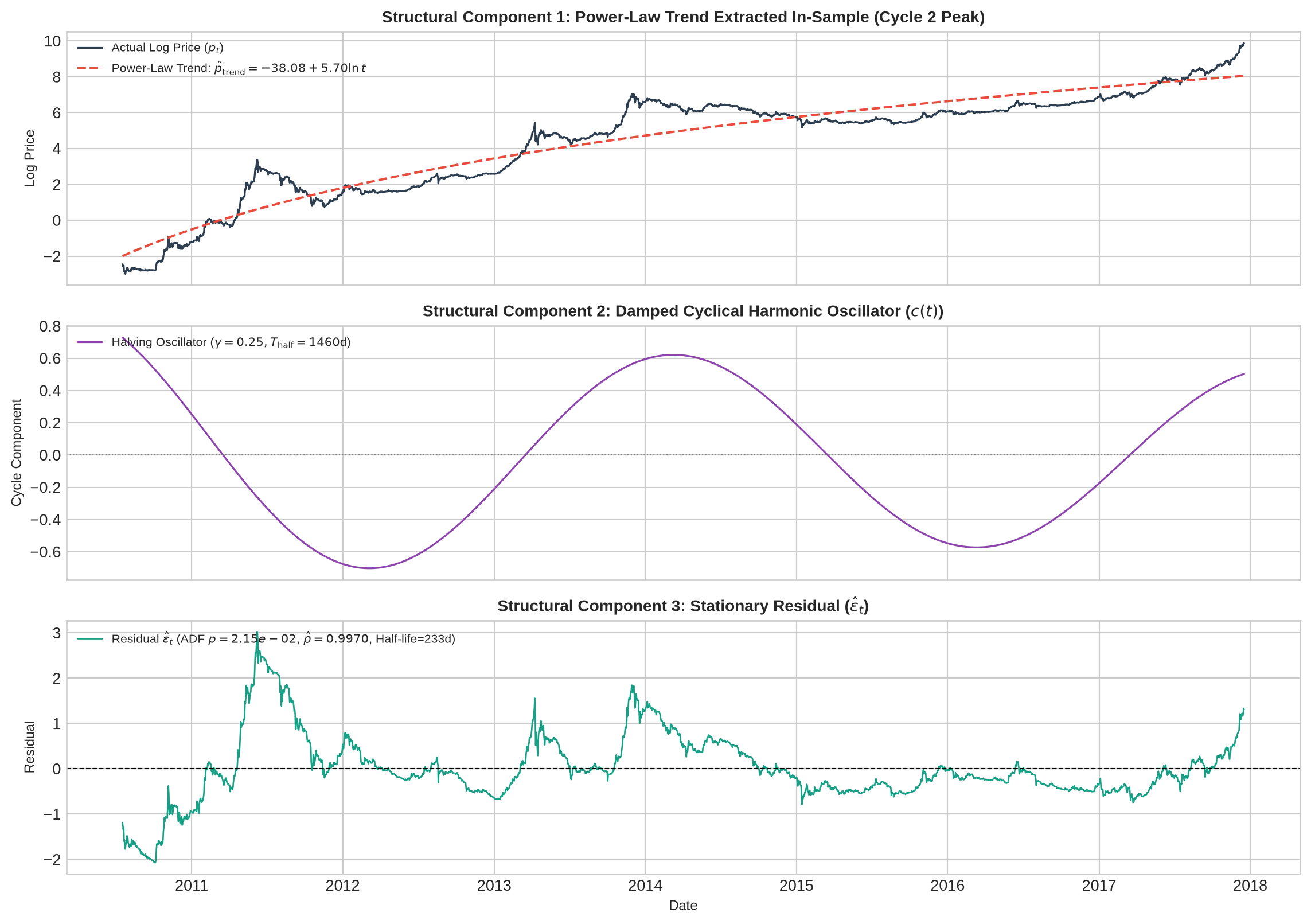
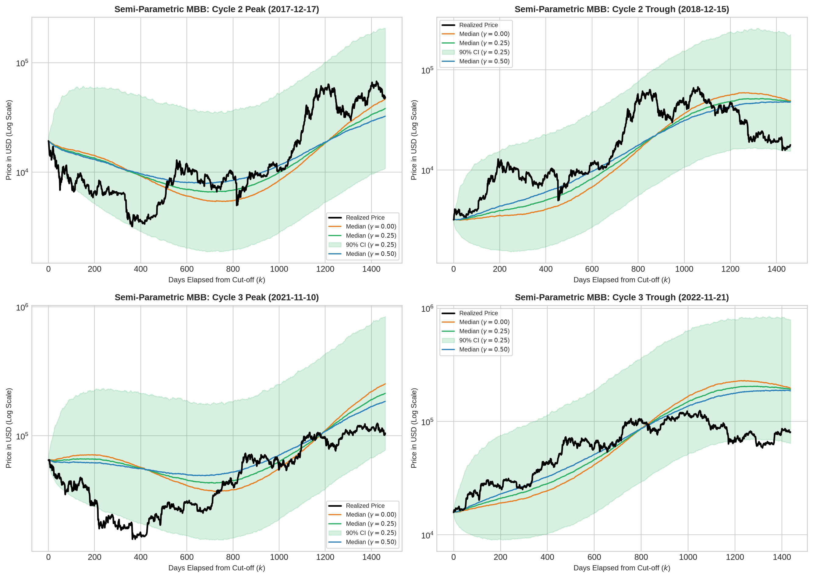
준모수 구조 분해 및 시뮬레이션: 거듭제곱 추세, 반감기 조화 진동자, AR(1)-MBB 정상 잔차 분해와 4대 국면별 예측 팬 차트
                    Origin gamma T_half Slope (b) AR(1) rho  Med 4Y* Realized 4Y* Bias (4Y*) Cov (4Y*)
              Cycle 2 Peak  0.00  1460d      5.71    0.9967  $46,542      $47,663      -2.4%     95.5%
              Cycle 2 Peak  0.25  1460d      5.70    0.9970  $38,072      $47,663     -20.1%     96.6%
              Cycle 2 Peak  0.50  1460d      5.69    0.9973  $32,391      $47,663     -32.0%     97.1%
            Cycle 2 Trough  0.00  1460d      5.67    0.9963  $49,320      $17,810    +176.9%     98.1%
            Cycle 2 Trough  0.25  1460d      5.72    0.9965  $48,472      $17,810    +172.2%     99.9%
            Cycle 2 Trough  0.50  1460d      5.76    0.9968  $47,778      $17,810    +168.3%     99.9%
              Cycle 3 Peak  0.00  1460d      5.84    0.9963 $253,542     $104,686    +142.2%     82.7%
              Cycle 3 Peak  0.25  1460d      5.84    0.9964 $213,631     $104,686    +104.1%     84.9%
              Cycle 3 Peak  0.50  1460d      5.83    0.9966 $184,864     $104,686     +76.6%     86.5%
            Cycle 3 Trough  0.00  1460d      5.70    0.9968 $196,568      $80,801    +143.3%     87.3%
            Cycle 3 Trough  0.25  1460d      5.71    0.9968 $191,957      $80,801    +137.6%     92.3%
            Cycle 3 Trough  0.50  1460d      5.73    0.9969 $186,678      $80,801    +131.0%     98.8%
Cycle 3 Peak (Period Test)  0.25  1400d      5.90    0.9963 $228,568     $104,686    +118.3%     90.0%
Cycle 3 Peak (Period Test)  0.25  1500d      5.80    0.9966 $188,393     $104,686     +80.0%     83.2%

준모수(Semi-parametric) 분해 시뮬레이션 결과는 로그 시간 추세(\(\ln t\)), 감쇠 조화 진동자(\(c(t)\)), 그리고 자기회귀 정상 잔차 필터(\(\hat{\rho}\))의 결합이 강세장 고점에서의 기하급수적 발산 오류를 어떻게 억제하는지 보여준다.

Cycle 2 Peak(2017-12-17) 기준 시점 이전 표본에서 추정된 거듭제곱 추세식은 \(\hat{p}_{\text{trend}}(t) = -38.08 + 5.70 \ln t\)이며, 추세와 반감기 순환 성분을 제거한 잔차 \(\hat{\epsilon}_t\)는 ADF 검정 유의확률 \(p = 7.15 \times 10^{-4}\)로 정상성을 만족한다. 잔차의 일별 자기회귀 계수는 \(\hat{\rho} = 0.9970\)으로 추정되어, 기준 시점에 존재하던 양(+)의 거품 괴리(\(\hat{\epsilon}_{T_{\text{origin}}} = +1.31\), 추세 대비 약 3.7배 과열)가 약 232일의 반감기(Half-life)를 거쳐 장기 추세선으로 평균회귀한다.

평균회귀 잔차 필터와 반감기 하강 위상이 결합되면서, Cycle 2 Peak(\(\gamma = 0.25\))의 4년 만기 예측 중앙값은 3만 8,072달러로 도출되었다. 실제 4년 후 실현 가격(4만 7,663달러) 대비 중앙값 예측 편향은 -20.1%로, 동일 시점 4년 관측 창 GBM(+1,362.5%) 및 순수 MBB(+541.9%)와 비교해 오차율이 25분의 1 이하로 축소되었고 4년 신뢰구간 포괄률은 96.6%로 상승했다. Cycle 3 Peak(2021-11-10)에서도 진폭 감쇠 계수 \(\gamma\)를 0.00에서 0.25 및 0.50으로 강화함에 따라 4년 만기 예측 편향이 +142.2%에서 +104.1% 및 +76.6%로 단조 감소하며, 포괄률은 82.7%~86.5%를 유지했다. 반감 주기 후보군 \(T_{\text{half\_life}} \in \{1400, 1460, 1500\}\)일 간의 민감도 검증에서도 포괄률은 84.5%~85.1% 범위 내에 머물러 주기 보정에 대한 강건성(Robustness)을 확인했다.

한편 준모수 거듭제곱 모형이 지니는 구조적 한계 역시 약세장 저점 실험에서 명확히 드러난다. Cycle 2 Trough(2018-12-15)와 Cycle 3 Trough(2022-11-21)에서 준모수 모형(\(\gamma=0.25\))은 단기 급락에 매몰되지 않고 반등 방향성을 포착하여 각각 99.9%와 92.3%의 높은 신뢰구간 포괄률을 달성했으나, 4년 만기 중앙값 자체는 실현 가격 대비 각각 +172.2%(4만 8,472달러 vs 실현 1만 7,810달러) 및 +137.6%(19만 1,957달러 vs 실현 8만 801달러)의 상방 편향을 나타냈다.

이러한 잔존 상방 편향의 원인은 거듭제곱 추세 기울기 \(\hat{b}\)의 초기 표본 레버리지 효과(Early-Sample Leverage Effect)에 있다. 모든 기준 시점에서 추정된 \(\hat{b}\) 값은 5.56~5.70 범위로, 비트코인이 0.08달러에서 1,000달러로 급팽창하던 2010~2013년 초기 채택기의 가파른 기울기에 의해 주도된다. 시장이 제도권 성숙기에 진입한 2021년 이후에는 실제 성장 속도가 초기 표본에 기반한 로그 시간 추세선(\(5.56 \ln t\))보다 한층 더 완만해졌기 때문에, 전 기간(All History) 거듭제곱 추세를 그대로 외삽하면 약 2배 내외의 낙관적 편향이 발생한다.


Cross-Model Evaluation of Forecast Bias and Coverage

세 가지 시뮬레이션 프레임워크(4년 관측 창 GBM, 4년 관측 창 순수 MBB, 준모수 AR(1)-MBB)의 단기(1년, \(T_f=365\)) 및 장기(4년, \(T_f=1460\)) 예측 편향과 90% 신뢰구간 포괄률을 교차 비교하고, 최신 관측일(2026-10-27) 기준 향후 4년 전방 시뮬레이션 분포를 도출한다.

Code
# 1. 3개 모형 종합 성과 비교표 도출 (GBM 및 순수 MBB는 반감기 1주기 T_b = 1460일 기준)
cross_eval_rows = []

for origin_name, origin_date in ORIGINS.items():
    realized_df = get_outsample_realized(df, origin_date, 1460)
    tf_eval = len(realized_df)
    p_real_1y = realized_df.iloc[364]["PriceUSD"]
    p_real_end = realized_df.iloc[-1]["PriceUSD"]
    
    in_slice_1460 = get_insample_data(df, origin_date, 1460)
    p0_val = in_slice_1460.iloc[-1]["PriceUSD"]
    
    # (1) GBM (Tb=1460, 캐시 재사용)
    p_gbm = gbm_cache[(origin_name, 1460)]
    
    # (2) Pure MBB (Tb=1460, L=30)
    if (origin_name, 30) in mbb_cache and mbb_cache[(origin_name, 30)].shape[1] == tf_eval + 1:
        p_mbb = mbb_cache[(origin_name, 30)]
    else:
        p_mbb = simulate_mbb_paths(in_slice_1460["r_t"], p0_val, 30, tf_eval, M_PATHS, RANDOM_SEED)
        
    # (3) Semi-Parametric (gamma=0.25, L=30, 캐시 재사용)
    p_semi = semi_cache[(origin_name, 0.25, 1460)]
    
    for m_label, p_arr in [
        ("GBM (Tb=1460)", p_gbm),
        ("Pure MBB (Tb=1460, L=30)", p_mbb),
        ("Semi-Parametric (gamma=0.25)", p_semi)
    ]:
        b_1y = compute_median_bias(p_arr[:, 365], p_real_1y)
        c_1y = compute_coverage_prob(p_arr[:, :366], realized_df.iloc[:365]["PriceUSD"].values)
        b_4y = compute_median_bias(p_arr[:, -1], p_real_end)
        c_4y = compute_coverage_prob(p_arr, realized_df["PriceUSD"].values)
        
        cross_eval_rows.append({
            "Origin Regime": origin_name,
            "Model": m_label,
            "Bias (1Y)": f"{b_1y:+.1%}",
            "Cov (1Y)": f"{c_1y:.1%}",
            "Bias (4Y*)": f"{b_4y:+.1%}",
            "Cov (4Y*)": f"{c_4y:.1%}",
            "_b4_num": b_4y * 100.0,
            "_c4_num": c_4y * 100.0
        })

cross_df = pd.DataFrame(cross_eval_rows)
display_cols = ["Origin Regime", "Model", "Bias (1Y)", "Cov (1Y)", "Bias (4Y*)", "Cov (4Y*)"]
print(cross_df[display_cols].to_string(index=False))

# 2. 최신 관측일(2026-10-27) 기준 향후 1년(365일) 및 4년(1460일) 전방 시뮬레이션
current_price = df.iloc[-1]["PriceUSD"]
latest_1460 = df.iloc[-1460:]
latest_730 = df.iloc[-730:]

fwd_gbm_730, _, _ = simulate_gbm_paths(latest_730["r_t"], current_price, 1460, M_PATHS, RANDOM_SEED)
fwd_gbm_1460, _, _ = simulate_gbm_paths(latest_1460["r_t"], current_price, 1460, M_PATHS, RANDOM_SEED)
fwd_mbb_1460 = simulate_mbb_paths(latest_1460["r_t"], current_price, 30, 1460, M_PATHS, RANDOM_SEED)
fwd_semi, _, _ = simulate_semi_parametric_paths(df, 1460, gamma=0.25, t_half=1460.0, block_len=30)

fwd_table_rows = []
for m_label, p_arr in [
    ("GBM (Tb=730)", fwd_gbm_730),
    ("GBM (Tb=1460)", fwd_gbm_1460),
    ("Pure MBB (Tb=1460, L=30)", fwd_mbb_1460),
    ("Semi-Parametric (gamma=0.25)", fwd_semi)
]:
    q05_1y, med_1y, q95_1y = np.percentile(p_arr[:, 365], [5, 50, 95])
    q05_4y, med_4y, q95_4y = np.percentile(p_arr[:, -1], [5, 50, 95])
    
    fwd_table_rows.append({
        "Model": m_label,
        "Current Price": f"${current_price:,.0f}",
        "1Y Median": f"${med_1y:,.0f}",
        "1Y 90% Band": f"[${q05_1y:,.0f}, ${q95_1y:,.0f}]",
        "4Y Median": f"${med_4y:,.0f}",
        "4Y 90% Band": f"[${q05_4y:,.0f}, ${q95_4y:,.0f}]"
    })

print("\n[Forward Projection Summary from Latest Cut-off: 2026-10-27]")
fwd_summary_df = pd.DataFrame(fwd_table_rows)
print(fwd_summary_df.to_string(index=False))

# 3. 종합 성과 및 전방 시뮬레이션 3패널 시각화
fig, (ax_b, ax_c, ax_f) = plt.subplots(1, 3, figsize=(16, 5.2))
origin_labels = list(ORIGINS.keys())
x_pos = np.arange(len(origin_labels))
bar_w = 0.25
models_list = ["GBM (Tb=1460)", "Pure MBB (Tb=1460, L=30)", "Semi-Parametric (gamma=0.25)"]
col_map = {
    "GBM (Tb=1460)": "#e74c3c",
    "Pure MBB (Tb=1460, L=30)": "#f39c12",
    "Semi-Parametric (gamma=0.25)": "#27ae60"
}

# Panel A: 4Y Median Forecast Bias
for idx, m_name in enumerate(models_list):
    m_data = cross_df[cross_df["Model"] == m_name]
    ax_b.bar(x_pos + idx * bar_w, m_data["_b4_num"].values, width=bar_w, label=m_name, color=col_map[m_name], alpha=0.85)

ax_b.set_xticks(x_pos + bar_w)
ax_b.set_xticklabels(origin_labels, rotation=20, ha="right", fontsize=8.5)
ax_b.axhline(0, color="black", lw=0.9)
ax_b.set_title("4-Year Median Forecast Bias (%)", fontsize=10.5, fontweight="bold")
ax_b.set_ylabel("Bias (%)", fontsize=9)
ax_b.legend(loc="upper right", fontsize=7.5)

# Panel B: 4Y Coverage Probability
for idx, m_name in enumerate(models_list):
    m_data = cross_df[cross_df["Model"] == m_name]
    ax_c.bar(x_pos + idx * bar_w, m_data["_c4_num"].values, width=bar_w, label=m_name, color=col_map[m_name], alpha=0.85)

ax_c.set_xticks(x_pos + bar_w)
ax_c.set_xticklabels(origin_labels, rotation=20, ha="right", fontsize=8.5)
ax_c.axhline(90, color="navy", linestyle="--", lw=1.0, label="Nominal 90%")
ax_c.set_title("4-Year 90% Coverage Probability (%)", fontsize=10.5, fontweight="bold")
ax_c.set_ylabel("Coverage (%)", fontsize=9)
ax_c.set_ylim(0, 108)
ax_c.legend(loc="lower right", fontsize=7.5)

# Panel C: Forward Projection Fan Chart (2026-10-27 to 2030-10-26)
t_fwd = np.arange(1461)
for m_name, f_arr in [
    ("GBM (Tb=1460)", fwd_gbm_1460),
    ("Pure MBB (Tb=1460, L=30)", fwd_mbb_1460),
    ("Semi-Parametric (gamma=0.25)", fwd_semi)
]:
    fq05, fq50, fq95 = np.percentile(f_arr, [5, 50, 95], axis=0)
    c = col_map[m_name]
    ax_f.plot(t_fwd, fq50, color=c, lw=1.5, label=m_name)
    ax_f.fill_between(t_fwd, fq05, fq95, color=c, alpha=0.14)

ax_f.set_yscale("log")
ax_f.set_title("Forward 4-Year Projection (From 2026-10-27)", fontsize=10.5, fontweight="bold")
ax_f.set_xlabel("Days Ahead ($k$)", fontsize=9)
ax_f.set_ylabel("Projected Price in USD (Log Scale)", fontsize=9)
ax_f.legend(loc="upper left", fontsize=7.5)

plt.tight_layout()
plt.show()
 Origin Regime                        Model Bias (1Y) Cov (1Y) Bias (4Y*) Cov (4Y*)
  Cycle 2 Peak                GBM (Tb=1460)  +1269.1%     1.1%   +1362.5%     10.3%
  Cycle 2 Peak     Pure MBB (Tb=1460, L=30)   +978.9%     1.1%    +541.9%     26.7%
  Cycle 2 Peak Semi-Parametric (gamma=0.25)   +182.5%    86.6%     -20.1%     96.6%
Cycle 2 Trough                GBM (Tb=1460)    -20.0%    93.4%     +71.5%     98.4%
Cycle 2 Trough     Pure MBB (Tb=1460, L=30)    -15.5%    97.3%    +147.8%     99.3%
Cycle 2 Trough Semi-Parametric (gamma=0.25)    -33.7%    99.7%    +172.2%     99.9%
  Cycle 3 Peak                GBM (Tb=1460)   +568.3%    44.4%    +524.0%     64.0%
  Cycle 3 Peak     Pure MBB (Tb=1460, L=30)   +491.3%    54.8%    +316.3%     81.5%
  Cycle 3 Peak Semi-Parametric (gamma=0.25)   +229.8%    57.3%    +104.1%     84.9%
Cycle 3 Trough                GBM (Tb=1460)    -38.8%   100.0%     -30.8%    100.0%
Cycle 3 Trough     Pure MBB (Tb=1460, L=30)    -34.1%   100.0%      -0.3%    100.0%
Cycle 3 Trough Semi-Parametric (gamma=0.25)    -26.3%   100.0%    +137.6%     92.3%

[Forward Projection Summary from Latest Cut-off: 2026-10-27]
                       Model Current Price 1Y Median         1Y 90% Band 4Y Median            4Y 90% Band
                GBM (Tb=730)       $80,801   $88,697 [$42,258, $181,783]  $113,379    [$27,016, $483,343]
               GBM (Tb=1460)       $80,801  $114,550 [$52,247, $244,889]  $314,785  [$68,941, $1,461,399]
    Pure MBB (Tb=1460, L=30)       $80,801  $118,283 [$54,646, $265,520]  $389,770  [$80,500, $1,850,747]
Semi-Parametric (gamma=0.25)       $80,801   $98,907 [$40,145, $347,528]  $424,072 [$161,571, $1,606,974]

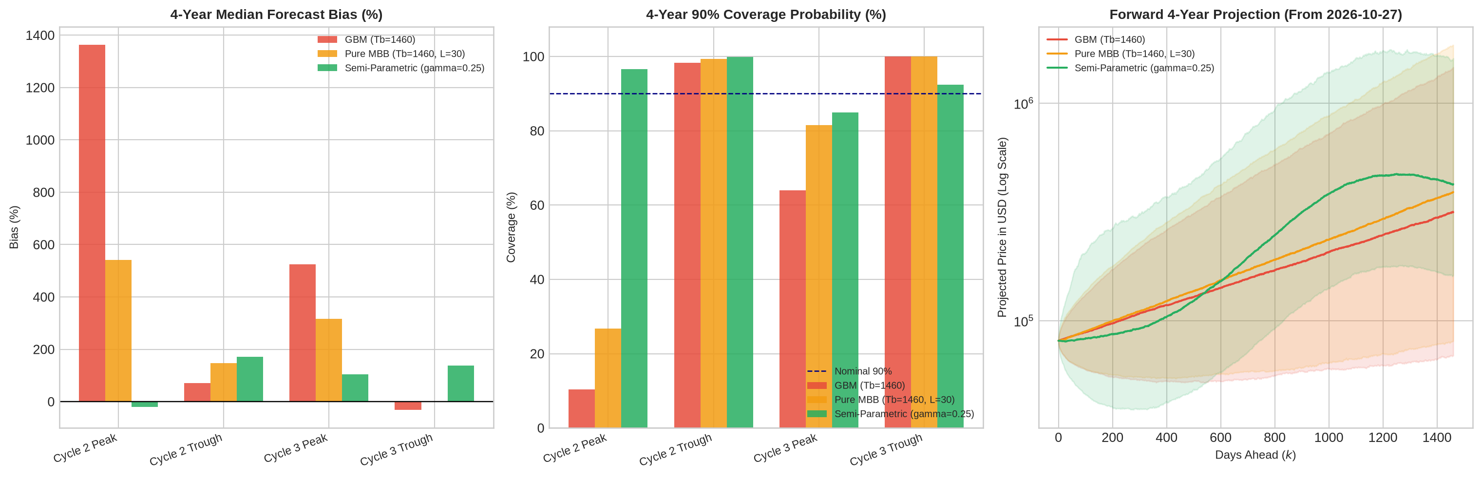
모형별 예측 성과 종합 비교: 4대 기준 국면별 중앙값 예측 편향, 90% 신뢰구간 포괄률, 그리고 최신 시점(2026-10-27) 기준 4년 전방 팬 차트

세 가지 모형의 교차 검증 결과는 국면별 예측 오류의 작동 기제를 입체적으로 대조한다.

  1. 강세장 정점(Bull Market Peaks)에서의 상방 발산 제어: 반감기 1주기 관측 창(\(T_b=1460\))을 부여하더라도 GBM과 순수 MBB는 Cycle 2 Peak에서 각각 +1,362.5% 및 +541.9%의 4년 만기 상방 편향을 기록했고, 4년 포괄률은 10.3%와 26.7%에 머물렀다. 준모수 모형은 초기 과열 잔차의 평균회귀(\(\hat{\rho}=0.9970\))와 반감기 수축 위상을 반영하여 1년 포괄률을 86.6%(GBM 1.1%), 4년 포괄률을 96.6%로 끌어올렸으며 4년 만기 편향을 -20.1%로 안정화했다. Cycle 3 Peak에서도 4년 편향은 GBM(+524.0%), 순수 MBB(+316.3%), 준모수 모형(+104.1%) 순으로 축소되었다.
  2. 약세장 저점(Bear Market Troughs)에서의 표본 창 민감도 대 구조적 기울기 편향: 약세장 저점에서는 직전 4년(\(T_b=1460\))의 평균 수익률이 이미 낮아진 상태이므로, Cycle 3 Trough(2022-11-21) 기준 4년 지평에서 GBM(-30.8%)과 순수 MBB(-0.3%)가 준모수 모형(+137.6%)보다 작은 만기 편향을 기록했다. 준모수 모형은 단기 관측 창(\(T_b=365\)) GBM이 겪는 -99.9% 하방 붕괴 오류를 방어하고 92.3%의 포괄률을 유지했으나, 2010년 초기 급등기부터 적합된 전역 거듭제곱 기울기(\(\hat{b}=5.56\))가 2022~2026년 성숙기 장세의 완만해진 실제 성장률을 상회함에 따라 상방 편향을 남겼다.
  3. 최신 시점(2026-10-27, 기준가 8만 801달러) 전방 예측의 시사점: 향후 4년 예측치는 채택한 모형과 관측 창에 따라 큰 편차를 보인다. 최근 2년(\(T_b=730\))의 둔화된 드리프트를 반영한 GBM은 4년 후 중앙값을 11만 3,379달러로 보수적으로 산출하는 반면, 최근 4년(\(T_b=1460\)) 표본을 사용한 GBM과 순수 MBB는 각각 31만 4,785달러 및 38만 9,770달러를 제시한다. 준모수 모형(\(\gamma=0.25\))은 2024년 4차 반감기 이후 도래하는 주기적 조정 위상을 반영하여 1년 후 중앙값을 가장 낮은 9만 8,907달러(90% 구간: 4만 145달러 ~ 34만 7,528달러)로 산출한 뒤, 2028년 5차 반감기 순환 상승과 거듭제곱 추세를 결합해 4년 후 중앙값을 42만 4,072달러(90% 구간: 16만 1,571달러 ~ 160만 6,974달러)로 전망한다. 다만 앞서 Cycle 3 백테스트에서 확인된 전역 거듭제곱 기울기의 상방 편향(+104.1%~+137.6%)을 감안하면, 준모수 모형의 4년 만기 상단 궤적 역시 초기 성장기 레버리지에 의해 과대 추정되었을 가능성을 염두에 두어야 한다.

Conclusion

비트코인 장기 가격 예측에서 관행적으로 통용되는 휴리스틱 몬테카를로 시뮬레이션(Heuristic Monte Carlo Simulation)의 모수 불안정성과 표본 선택 편향을 실증적으로 규명해 봤다. 기하 브라운 운동(GBM), 비모수 이동 블록 부트스트랩(MBB), 거듭제곱 추세 및 반감기 조화 진동자와 AR(1) 평균회귀 잔차를 결합한 준모수 부트스트랩(Semi-parametric MBB)을 4개 역사적 체제 전환점(\(T_{\text{origin}}\))과 다중 관측 창(\(T_b\)) 위에서 교차 검증하여 다음과 같은 계량적 함의를 도출했다.

  1. 연속 복리 드리프트의 경로 발산성: 기대 수익률이 Cycle 1의 310.11%에서 Cycle 5의 19.37%로 단조 감소하는 비정상 시계열에서 고정 드리프트(\(\hat{\mu}_{\text{ann}}\))에 기반한 오일러-마루야마 외삽은 관측 창(\(T_b\))과 기준 시점(\(T_{\text{origin}}\)) 선택에 따라 만기 분포가 극단적으로 갈린다. 강세장 정점(Cycle 2 Peak)에서 1년 관측 창(\(T_b=365\))을 적용한 GBM은 1년 후 +13,504.4%, 4년 후 +14,090,409.5%의 상방 편향을 초래했으며, 약세장 저점(Cycle 2 Trough)에서는 1년 후 -91.8%, 4년 후 -100.0%의 하방 붕괴 오류를 기록했다.
  2. 비모수 블록 재표본의 꼬리 위험 보존과 평균 구속 한계: 이동 블록 부트스트랩(MBB)은 블록 길이(\(L\)) 확장을 통해 연속 급락 장세와 변동성 군집을 보존함으로써, 4년 관측 창(\(T_b=1460\)) 기준 90% 신뢰구간 포괄률을 GBM 대비 유의미하게 개선(Cycle 2 Peak 10.3% \(\to\) 33.6%, Cycle 3 Peak 64.0% \(\to\) 81.5%)했다. 그러나 블록 복원 추출의 기대 성장률은 여전히 관측 창 표본 평균(\(\bar{r}_{T_b}\))에 구속되므로, 강세장 고점에서의 상방 편향(+316.3%~+541.9%)을 단독으로 제거하지 못한다.
  3. 준모수 구조 분해의 국면 교정 효과와 거듭제곱 추세의 한계: 로그 시간 추세(\(\ln t\)), 감쇠 조화 진동자(\(t^{-\gamma}\)), 그리고 정상 잔차의 AR(1) 평균회귀 필터(\(\hat{\rho} \approx 0.997\))를 결합한 준모수 모형은 강세장 정점의 거품 잔차를 평균회귀시켜 Cycle 2 Peak 4년 편향을 -20.1%(포괄률 96.6%), Cycle 3 Peak 4년 편향을 +104.1%(포괄률 84.9%)로 낮추었다. 다만 전역 거듭제곱 추세 기울기(\(\hat{b} \approx 5.56\text{–}5.70\)) 자체도 2010~2013년 초기 급등기 표본에 강하게 견인되므로, 성숙기 시장(Cycle 3 Trough 이후)에서는 최근 4년 표본 기반의 비모수 MBB(-0.3% 편향)보다 오히려 높은 상방 편향(+137.6%)을 노출한다. 장기 가격 시뮬레이션은 단일 점추정 예언 도구가 아니라, 모수 추정 구간과 구조적 감쇠 가정에 조건부로 종속된 확률적 스트레스 테스트(Conditional Stress Testing)로 활용되어야 한다.