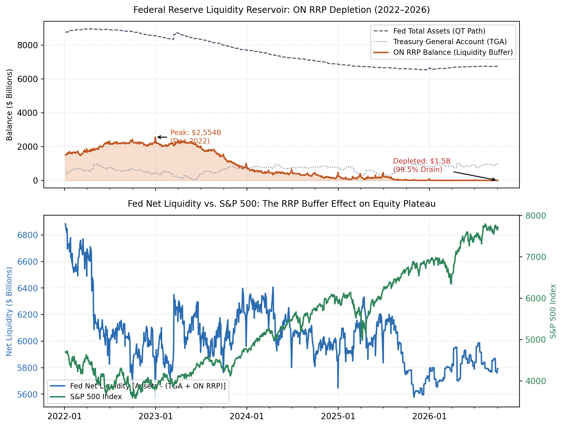
from pathlib import Path
import pandas as pd
import matplotlib.pyplot as plt
import matplotlib.dates as mdates

cache_path = Path('diary_liquidity.parquet')
if not cache_path.exists():
    cache_path = Path('posts/diary_liquidity.parquet')

if cache_path.exists():
    df = pd.read_parquet(cache_path)
else:
    import yfinance as yf
    rrp = pd.read_csv('https://fred.stlouisfed.org/graph/fredgraph.csv?id=RRPONTSYD')
    rrp.columns = ['Date', 'ON_RRP']
    rrp['Date'] = pd.to_datetime(rrp['Date'])
    rrp['ON_RRP'] = pd.to_numeric(rrp['ON_RRP'], errors='coerce')
    rrp = rrp.dropna().set_index('Date')

    walcl = pd.read_csv('https://fred.stlouisfed.org/graph/fredgraph.csv?id=WALCL')
    walcl.columns = ['Date', 'Total_Assets']
    walcl['Date'] = pd.to_datetime(walcl['Date'])
    walcl['Total_Assets'] = pd.to_numeric(walcl['Total_Assets'], errors='coerce') / 1000.0
    walcl = walcl.dropna().set_index('Date')

    tga = pd.read_csv('https://fred.stlouisfed.org/graph/fredgraph.csv?id=WTREGEN')
    tga.columns = ['Date', 'TGA']
    tga['Date'] = pd.to_datetime(tga['Date'])
    tga['TGA'] = pd.to_numeric(tga['TGA'], errors='coerce') / 1000.0
    tga = tga.dropna().set_index('Date')

    sp = yf.download('^GSPC', start='2022-01-01', end='2026-10-03', auto_adjust=True)['Close']
    sp = sp.rename(columns={'^GSPC': 'SP500'}) if isinstance(sp, pd.DataFrame) else sp.to_frame('SP500')

    df = pd.concat([walcl, tga, rrp], axis=1).sort_index().loc['2022-01-01':'2026-10-02'].ffill().dropna()
    df['Net_Liquidity'] = df['Total_Assets'] - (df['TGA'] + df['ON_RRP'])
    df = pd.concat([df, sp], axis=1).sort_index().loc['2022-01-01':'2026-10-02'].dropna()
    df.to_parquet('diary_liquidity.parquet')

fig, (ax1, ax2) = plt.subplots(2, 1, figsize=(9.5, 7.2), sharex=True, gridspec_kw={'height_ratios': [1, 1.15]})

# Panel 1: Fed Balance Sheet & ON RRP Depletion
ax1.plot(df.index, df['Total_Assets'], color='#4a5568', linestyle='--', linewidth=1.2, label='Fed Total Assets (QT Path)')
ax1.plot(df.index, df['TGA'], color='#718096', linestyle=':', linewidth=1.1, label='Treasury General Account (TGA)')
ax1.fill_between(df.index, df['ON_RRP'], color='#dd6b20', alpha=0.22)
ax1.plot(df.index, df['ON_RRP'], color='#c05621', linewidth=1.7, label='ON RRP Balance (Liquidity Buffer)')

ax1.set_ylabel('Balance ($ Billions)', fontsize=9)
ax1.set_title('Federal Reserve Liquidity Reservoir: ON RRP Depletion (2022–2026)', fontsize=10.5, pad=10)
ax1.grid(True, linestyle=':', alpha=0.5)
ax1.legend(loc='upper right', frameon=True, facecolor='white', edgecolor='#cccccc', fontsize=8.5)

peak_date = df['ON_RRP'].idxmax()
peak_val = df.loc[peak_date, 'ON_RRP']
ax1.annotate(f'Peak: ${peak_val:,.0f}B\n(Dec 2022)', xy=(peak_date, peak_val), xytext=(peak_date + pd.Timedelta(days=60), peak_val - 350),
             arrowprops=dict(facecolor='#c05621', arrowstyle='->', lw=1.1), fontsize=8.5, color='#c05621')

trough_date = df.index[-1]
trough_val = df.loc[trough_date, 'ON_RRP']
ax1.annotate(f'Depleted: ${trough_val:.1f}B\n(99.5% Drain)', xy=(trough_date, trough_val), xytext=(trough_date - pd.Timedelta(days=420), trough_val + 500),
             arrowprops=dict(facecolor='#e53e3e', arrowstyle='->', lw=1.1), fontsize=8.5, color='#c53030')

# Panel 2: Net Liquidity vs S&P 500
ax2_twin = ax2.twinx()
l1 = ax2.plot(df.index, df['Net_Liquidity'], color='#2b6cb0', linewidth=1.7, label='Fed Net Liquidity [Assets - (TGA + ON RRP)]')
l2 = ax2_twin.plot(df.index, df['SP500'], color='#2f855a', linewidth=1.7, label='S&P 500 Index')

ax2.set_ylabel('Net Liquidity ($ Billions)', color='#2b6cb0', fontsize=9)
ax2_twin.set_ylabel('S&P 500 Index', color='#2f855a', fontsize=9)
ax2.tick_params(axis='y', labelcolor='#2b6cb0')
ax2_twin.tick_params(axis='y', labelcolor='#2f855a')

ax2.set_title('Fed Net Liquidity vs. S&P 500: The RRP Buffer Effect on Equity Plateau', fontsize=10.5, pad=10)
ax2.grid(True, linestyle=':', alpha=0.5)

lines = l1 + l2
labels = [l.get_label() for l in lines]
ax2.legend(lines, labels, loc='lower left', frameon=True, facecolor='white', edgecolor='#cccccc', fontsize=8.5)

ax2.xaxis.set_major_locator(mdates.YearLocator())
ax2.xaxis.set_major_formatter(mdates.DateFormatter('%Y-%m'))
ax2.xaxis.set_minor_locator(mdates.MonthLocator(bymonth=[4, 7, 10]))

plt.tight_layout()
plt.show()