Pre, Main, and Post-Market Correlations: US Wishlist Stock Returns

미국 주요 주식 및 ETF의 세션별(장전·정규장·장후) 일간 수익률, VWAP 롤링 스무딩 및 극단치 제거 선형 상관관계 분석

Data

Author

gitSAM

Published

September 23, 2026

Code

import os
import time
import yfinance as yf
import duckdb
import numpy as np
import pandas as pd
import matplotlib.pyplot as plt
import seaborn as sns
from pathlib import Path

# Matplotlib & Seaborn 시각화 기본 스타일 설정
plt.style.use('seaborn-v0_8-whitegrid' if 'seaborn-v0_8-whitegrid' in plt.style.available else 'default')
plt.rcParams['font.family'] = 'DejaVu Sans'
plt.rcParams['axes.unicode_minus'] = False

1 서론

미국 증권시장의 하루 거래는 거래소 규정에 따라 3개의 서로 다른 유동성 세션으로 구성된다. 본 연구에서는 정규장 개장 30분 전부터 유입되는 수급 선반영 효과를 포착하고 연산 효율을 높이기 위해 1시간봉(1Hour Bar) 체계를 적용하며, 정규장 시작 기준점을 09:00(ET) 로 정의한다.

프리마켓 (Pre-Market, 04:00 ~ 09:00 ET):

주요 거시 경제지표(CPI, 고용보고서 등 08:30 ET 발표)와 기업 실적(장 개시 전 발표)이 1차 반영되는 구간.
04:00~08:00 시간대 캔들을 포함하여 09:00 시점까지의 장전 가격 변동 집계.

정규장 (Main Market, 09:00 ~ 16:00 ET):

개장 직전 30분(09:00~09:30)의 초반 유동성 및 장 개시 후 전 세계 수급이 집중되는 중심 세션.
09:00 시가부터 16:00 장 마감 종가까지의 수익률을 측정.

포스트마켓 (Post-Market / After-Hours, 16:00 ~ 20:00 ET):

장 마감 직후 분기 실적 발표(Earnings Release) 및 컨퍼런스 콜 이벤트가 집중 반영되는 구간.

1.1 분석 가설

가설 1 (Pre \(\rightarrow\) Main 과열/반전 여부): 프리마켓의 가격 급등락이 정규장 개장 후에도 연속적인 모멘텀을 형성하는가, 아니면 갭 채우기(Mean Reversion) 형태의 역상관을 나타내는가?
가설 2 (Main \(\rightarrow\) Post 실적 및 뉴스 충격): 정규장의 일중 추세가 장 마감 후 시간외 거래로 전이되는 경향이 존재하는가?
가설 3 (Post \(\rightarrow\) Next Pre 오버나이트 전이): 전일 장후 실적 충격이 익일 장전 프리마켓까지 유지되는 상관계수는 어느 정도인가?
가설 4 (VWAP 롤링 스무딩 효과): 단순 종가 대신 세션별 거래량 가중 평균 가격(VWAP)과 롤링 윈도우(\(n=20\)일)를 결합했을 때 노이즈가 제거된 본질적 수급 동조화가 나타나는가?
가설 5 (극단적 이벤트 데이의 왜곡): 실적 발표 및 FOMC 등 절대 수익률 상위 1%의 극단치 날짜를 제외(Trimmed)했을 때, 평상시 세션 간 선형 상관관계는 어떻게 변모하는가?

2 분석 대상

시장 대표 ETF 3종과 변동성이 높고 시간외 실적 발표 민감도가 큰 테크 대형주 7종을 유니버스로 설정한다.

Type	Ticker	Name	특징
Index	`SPY`	SPDR S&P 500 ETF Trust	시장 전체 벤치마크
	`QQQ`	Invesco QQQ Trust (Nasdaq 100)	테크 대형주 집중 지수
	`DIA`	SPDR Dow Jones Industrial Average	전통 대형 우량주 지수
HW	`NVDA`	NVIDIA Corporation	AI 인프라 대장주
	`AMD`	Advanced Micro Devices	반도체 고베타 종목
	`MU`	Micron Technology	메모리 사이클 대표주
	`DELL`	Dell Technologies	서버/AI 하드웨어 대표주
SW	`PLTR`	Palantir Technologies	리테일/기관 수급 집중 종목
	`NET`	Cloudflare	클라우드 보안/인프라 성장주
	`META`	Meta Platforms	빅테크 플랫폼, 실적 발표 민감주

3 데이터 수집

3.1 데이터 수집 환경 및 사전 준비

데이터 소스: Yahoo Finance (yfinance API, 미국 전 거래소 통합 테이프)
수집 주기: 1시간봉(1Hour intraday bar, prepost=True)
관측 기간: 최근 730일 (약 2개년, 미국 거래소 시간외 체결 완벽 보존)
저장소: ZSTD 압축 Parquet 파일 (market_stock_yfinance.parquet, 단 1.9MB)

3.2 세션별 시점 및 수익률 정의

미국 동부시간(US Eastern Time, ET) 기준 1시간봉 타임스탬프를 매핑하여 정의한다. 개장 30분 전(09:00 ET)부터 장 초반 유동성이 유입되는 현실을 감안하여 09:00 시점을 프리마켓의 종가이자 정규장의 시가로 활용한다.

3.2.1 단순 가격(Close) 기반 수익률

\[ \text{Pre-Market Return } (R_{\text{pre}, t}) = \frac{P_{09:00, t} - P_{04:00, t}}{P_{04:00, t}} \]

\[ \text{Main-Market Return } (R_{\text{main}, t}) = \frac{P_{16:00, t} - P_{09:00, t}}{P_{09:00, t}} \]

\[ \text{Post-Market Return } (R_{\text{post}, t}) = \frac{P_{20:00, t} - P_{16:00, t}}{P_{16:00, t}} \]

\[ \text{Overnight Return } (R_{\text{overnight}, t}) = \frac{P_{04:00, t} - P_{20:00, t-1}}{P_{20:00, t-1}} \]

3.2.2 세션별 VWAP (Volume-Weighted Average Price) 산출

단순 체결 종가 대신 1시간봉의 대표가격(Typical Price, \(\bar{P}\))과 거래량(\(V\))을 가중 결합하여 세션별 실질 평균 체결 단가를 산출한다.

\[ \bar{P}_{k} = \frac{\text{High}_{k} + \text{Low}_{k} + \text{Close}_{k}}{3} \]

\[ \text{Session VWAP}_{s, t} = \frac{\sum_{k \in s} \bar{P}_{k} \times V_{k}}{\sum_{k \in s} V_{k}} \quad (s \in \{\text{pre}, \text{main}, \text{post}\}) \]

세션별 VWAP 수익률은 직전 세션(또는 당일 기준 세션)의 VWAP 대비 변동률로 정의한다:

\[ R^{\text{vwap}}_{\text{pre}, t} = \frac{\text{VWAP}_{\text{pre}, t} - \text{VWAP}_{\text{post}, t-1}}{\text{VWAP}_{\text{post}, t-1}}, \quad R^{\text{vwap}}_{\text{main}, t} = \frac{\text{VWAP}_{\text{main}, t} - \text{VWAP}_{\text{pre}, t}}{\text{VWAP}_{\text{pre}, t}}, \quad R^{\text{vwap}}_{\text{post}, t} = \frac{\text{VWAP}_{\text{post}, t} - \text{VWAP}_{\text{main}, t}}{\text{VWAP}_{\text{main}, t}} \]

3.3 데이터 파이프라인 및 Parquet 캐싱

Git 저장소 용량을 최소화(23.8MB \(\rightarrow\) 1.9MB, 92% 절감)하기 위해 ZSTD 압축 Parquet 포맷으로 영구 저장하고, DuckDB 인메모리 엔진을 통해 디스크에서 직접 무감압 네이티브 뷰(raw_bars)로 연동한다. 파일 Lock 충돌 없이 VSCode 인터랙티브와 Quarto 렌더링 양쪽에서 즉각 실행된다.

Code

# 1. 대상 유니버스 정의
SYMBOLS = ['SPY', 'QQQ', 'DIA', 'NVDA', 'MU', 'AMD', 'DELL', 'PLTR', 'NET', 'META']

# 2. 실행 환경(VSCode 인터랙티브 루트 cwd 또는 Quarto render의 posts/ cwd)에 맞게 Parquet 경로 자동 판별
PQ_NAME = "market_stock_yfinance.parquet"
PQ_PATH = Path(PQ_NAME).resolve() if Path(PQ_NAME).exists() or Path(".").resolve().name == "posts" else (Path("posts") / PQ_NAME).resolve()

# 3. Parquet 캐시가 없으면 yfinance 일괄 다운로드 후 저장 (최초 1회 실행)
if not PQ_PATH.exists():
    print("yfinance를 통해 10개 종목의 최근 730일 1시간봉(Pre/Post 포함) 일괄 다운로드 중...")
    t0 = time.time()
    raw = yf.download(SYMBOLS, period='730d', interval='1h', prepost=True, group_by='ticker', progress=False)
    
    dfs = []
    for sym in SYMBOLS:
        df_s = raw[sym].dropna(subset=['Close']).copy().reset_index()
        time_col = 'Datetime' if 'Datetime' in df_s.columns else 'Date'
        df_s = df_s.rename(columns={time_col: 'timestamp', 'Open': 'open', 'High': 'high', 'Low': 'low', 'Close': 'close', 'Volume': 'volume'})
        df_s['symbol'] = sym
        df_s = df_s[['symbol', 'timestamp', 'open', 'high', 'low', 'close', 'volume']]
        dfs.append(df_s)
        
    combined_df = pd.concat(dfs, ignore_index=True)
    
    # DuckDB를 통해 ZSTD 압축 Parquet로 즉시 저장
    duckdb.connect().execute(f"COPY (SELECT * FROM combined_df) TO '{PQ_PATH.as_posix()}' (FORMAT PARQUET, COMPRESSION 'ZSTD')")
    print(f"다운로드 및 Parquet 압축 저장 완료: 총 {len(combined_df):,}건 (소요시간: {time.time()-t0:.2f}초).")

# 4. DuckDB 인메모리 연결 및 Parquet 직접 뷰 생성 (Lock 충돌 방지 및 초고속 I/O)
con = duckdb.connect()
con.execute(f"CREATE OR REPLACE VIEW raw_bars AS SELECT * FROM '{PQ_PATH.as_posix()}'")

# 수집 현황 요약
df_summary = con.execute("""
SELECT symbol, 
       COUNT(*) AS bar_count, 
       MIN(timestamp) AS start_ts, 
       MAX(timestamp) AS end_ts 
FROM raw_bars 
GROUP BY symbol 
ORDER BY symbol
""").df()
df_summary

	symbol	bar_count	start_ts	end_ts
0	AMD	12068	2023-10-25 17:00:00+09:00	2026-09-23 21:00:00+09:00
1	DELL	12052	2023-10-25 20:00:00+09:00	2026-09-23 21:00:00+09:00
2	DIA	12097	2023-10-25 17:00:00+09:00	2026-09-23 21:00:00+09:00
3	META	12068	2023-10-25 17:00:00+09:00	2026-09-23 21:00:00+09:00
4	MU	12067	2023-10-25 17:00:00+09:00	2026-09-23 21:00:00+09:00
5	NET	12052	2023-10-25 17:00:00+09:00	2026-09-23 21:00:00+09:00
6	NVDA	12068	2023-10-25 17:00:00+09:00	2026-09-23 21:00:00+09:00
7	PLTR	12077	2023-10-25 17:00:00+09:00	2026-09-23 21:56:00+09:00
8	QQQ	12068	2023-10-25 17:00:00+09:00	2026-09-23 21:00:00+09:00
9	SPY	12098	2023-10-25 17:00:00+09:00	2026-09-23 21:00:00+09:00

4 방법론 및 결과 분석

4.1 세션별 지표 집계 및 DuckDB 가공 (`session_features`)

DuckDB의 SQL 엔진을 활용하여 뉴욕 현지시간 기준 각 세션의 시초가, 종가, 대표가격(\(\bar{P} = \frac{H+L+C}{3}\)), 거래량 가중 평균 가격(VWAP)을 일별로 산출한다.

Code

# 1. 1시간봉을 America/New_York 타임존으로 변환하고 세션 라벨(pre, main, post) 부여
con.execute("""
CREATE OR REPLACE TABLE session_bars AS
SELECT 
    symbol,
    timezone('America/New_York', timestamp) AS ts_ny,
    CAST(timezone('America/New_York', timestamp) AS DATE) AS trade_date,
    date_part('hour', timezone('America/New_York', timestamp)) AS hr,
    open, high, low, close, volume,
    (high + low + close) / 3.0 AS typical_price,
    ((high + low + close) / 3.0) * volume AS tp_vol,
    CASE 
        WHEN date_part('hour', timezone('America/New_York', timestamp)) >= 4 
         AND date_part('hour', timezone('America/New_York', timestamp)) < 9 THEN 'pre'
        WHEN date_part('hour', timezone('America/New_York', timestamp)) >= 9 
         AND date_part('hour', timezone('America/New_York', timestamp)) < 16 THEN 'main'
        WHEN date_part('hour', timezone('America/New_York', timestamp)) >= 16 
         AND date_part('hour', timezone('America/New_York', timestamp)) < 20 THEN 'post'
        ELSE 'other'
    END AS session
FROM raw_bars
WHERE session != 'other';
""")

# 2. 일별/세션별 집계: Open, Close, Volume, VWAP 산출
con.execute("""
CREATE OR REPLACE TABLE daily_sessions AS
SELECT 
    symbol,
    trade_date,
    session,
    arg_min(open, ts_ny) AS session_open,
    arg_max(close, ts_ny) AS session_close,
    SUM(volume) AS session_vol,
    CASE 
        WHEN SUM(volume) > 0 THEN SUM(tp_vol) / SUM(volume)
        ELSE arg_max(close, ts_ny)
    END AS session_vwap
FROM session_bars
GROUP BY symbol, trade_date, session;
""")

# 3. 피벗 및 수익률 계산 테이블 생성
con.execute("""
CREATE OR REPLACE TABLE session_returns AS
WITH pivoted AS (
    SELECT 
        symbol,
        trade_date,
        MAX(CASE WHEN session = 'pre' THEN session_open END) AS pre_open,
        MAX(CASE WHEN session = 'pre' THEN session_close END) AS pre_close,
        MAX(CASE WHEN session = 'pre' THEN session_vwap END) AS pre_vwap,
        MAX(CASE WHEN session = 'pre' THEN session_vol END) AS pre_vol,

        MAX(CASE WHEN session = 'main' THEN session_open END) AS main_open,
        MAX(CASE WHEN session = 'main' THEN session_close END) AS main_close,
        MAX(CASE WHEN session = 'main' THEN session_vwap END) AS main_vwap,
        MAX(CASE WHEN session = 'main' THEN session_vol END) AS main_vol,

        MAX(CASE WHEN session = 'post' THEN session_open END) AS post_open,
        MAX(CASE WHEN session = 'post' THEN session_close END) AS post_close,
        MAX(CASE WHEN session = 'post' THEN session_vwap END) AS post_vwap,
        MAX(CASE WHEN session = 'post' THEN session_vol END) AS post_vol
    FROM daily_sessions
    GROUP BY symbol, trade_date
)
SELECT 
    symbol,
    trade_date,
    -- 가격 기반 수익률
    (pre_close - pre_open) / NULLIF(pre_open, 0) AS ret_pre_price,
    (main_close - pre_close) / NULLIF(pre_close, 0) AS ret_main_price,
    (post_close - main_close) / NULLIF(main_close, 0) AS ret_post_price,
    LAG(post_close) OVER (PARTITION BY symbol ORDER BY trade_date) AS prev_post_close,
    (pre_open - LAG(post_close) OVER (PARTITION BY symbol ORDER BY trade_date)) 
        / NULLIF(LAG(post_close) OVER (PARTITION BY symbol ORDER BY trade_date), 0) AS ret_overnight_price,

    -- VWAP 기반 수익률
    LAG(post_vwap) OVER (PARTITION BY symbol ORDER BY trade_date) AS prev_post_vwap,
    (pre_vwap - LAG(post_vwap) OVER (PARTITION BY symbol ORDER BY trade_date)) 
        / NULLIF(LAG(post_vwap) OVER (PARTITION BY symbol ORDER BY trade_date), 0) AS ret_pre_vwap,
    (main_vwap - pre_vwap) / NULLIF(pre_vwap, 0) AS ret_main_vwap,
    (post_vwap - main_vwap) / NULLIF(main_vwap, 0) AS ret_post_vwap,
    
    pre_vol, main_vol, post_vol
FROM pivoted
ORDER BY symbol, trade_date;
""")

df_returns = con.execute("SELECT * FROM session_returns WHERE ret_pre_price IS NOT NULL AND ret_main_price IS NOT NULL").df()
print(f"가공 완료: 총 {len(df_returns)}행의 세션별 수익률 데이터 적재됨.")
df_returns.head(3)

가공 완료: 총 7269행의 세션별 수익률 데이터 적재됨.

	symbol	trade_date	ret_pre_price	ret_main_price	ret_post_price	prev_post_close	ret_overnight_price	prev_post_vwap	ret_pre_vwap	ret_main_vwap	ret_post_vwap	main_vol
0	AMD	2023-10-25	-0.001486	-0.047024	-0.023006	NaN	NaN	NaN	NaN	-0.031879	-0.038290	49393893.0
1	AMD	2023-10-26	0.015956	-0.013176	0.020081	93.85	-0.005008	93.85	0.010868	-0.004300	0.010987	46824869.0
2	AMD	2023-10-27	0.000524	0.009733	-0.002384	95.50	0.000000	95.50	0.000524	0.007870	-0.000539	49993534.0

4.2 단순 가격 일간 수익률 간 선형 상관관계 (Baseline Correlation)

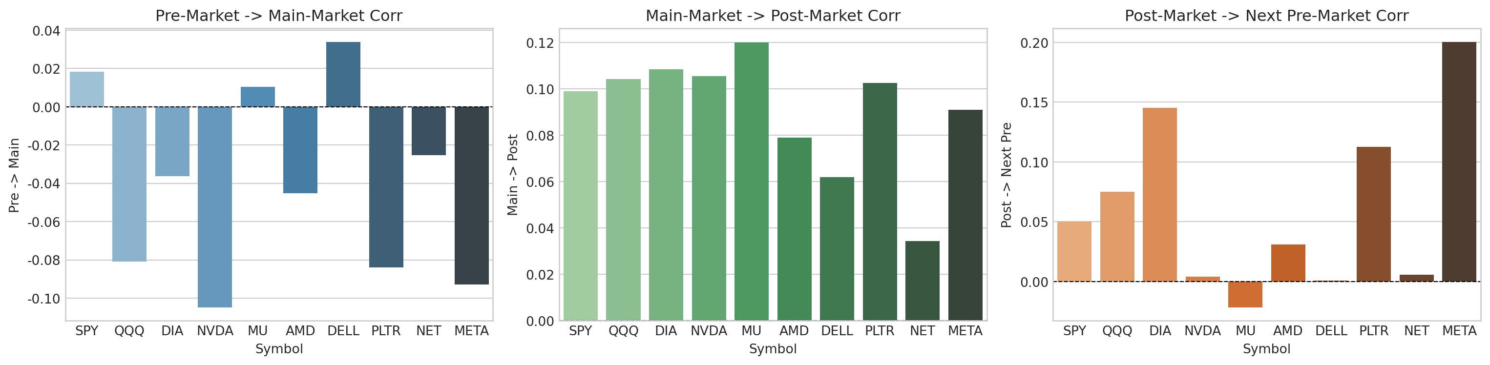
단순 체결가 기준으로 당일 장전과 정규장(Pre \(\rightarrow\) Main), 정규장과 장후(Main \(\rightarrow\) Post), 전일 장후와 익일 장전(Post \(\rightarrow\) Next Pre)의 피어슨 선형 상관계수(\(r\))를 산출한다.

Code

corr_list = []
for sym in SYMBOLS:
    df_s = df_returns[df_returns['symbol'] == sym].dropna(subset=['ret_pre_price', 'ret_main_price', 'ret_post_price']).copy()
    
    # 최소 관측치(30건 이상) 충족 여부 확인 후 상관계수 계산
    if len(df_s) >= 30:
        r_pre_main = df_s['ret_pre_price'].corr(df_s['ret_main_price'])
        r_main_post = df_s['ret_main_price'].corr(df_s['ret_post_price'])
        r_post_nextpre = df_s['ret_post_price'].shift(1).corr(df_s['ret_pre_price'])
    else:
        r_pre_main, r_main_post, r_post_nextpre = np.nan, np.nan, np.nan
    
    corr_list.append({
        'Symbol': sym,
        'Pre -> Main': r_pre_main,
        'Main -> Post': r_main_post,
        'Post -> Next Pre': r_post_nextpre
    })

df_corr_price = pd.DataFrame(corr_list).set_index('Symbol')

fig, axes = plt.subplots(1, 3, figsize=(16, 4))
sns.barplot(x=df_corr_price.index, y=df_corr_price['Pre -> Main'], hue=df_corr_price.index, ax=axes[0], palette='Blues_d', legend=False)
axes[0].set_title('Pre-Market -> Main-Market Corr')
axes[0].axhline(0, color='black', linestyle='--', linewidth=0.8)

sns.barplot(x=df_corr_price.index, y=df_corr_price['Main -> Post'], hue=df_corr_price.index, ax=axes[1], palette='Greens_d', legend=False)
axes[1].set_title('Main-Market -> Post-Market Corr')
axes[1].axhline(0, color='black', linestyle='--', linewidth=0.8)

sns.barplot(x=df_corr_price.index, y=df_corr_price['Post -> Next Pre'], hue=df_corr_price.index, ax=axes[2], palette='Oranges_d', legend=False)
axes[2].set_title('Post-Market -> Next Pre-Market Corr')
axes[2].axhline(0, color='black', linestyle='--', linewidth=0.8)

plt.tight_layout()
plt.show()

df_corr_price

	Pre -> Main	Main -> Post	Post -> Next Pre
Symbol
SPY	0.018231	0.098907	0.050287
QQQ	-0.080771	0.104128	0.074991
DIA	-0.036379	0.108516	0.145210
NVDA	-0.104767	0.105418	0.004054
MU	0.010541	0.120036	-0.021548
AMD	-0.045126	0.078967	0.030971
DELL	0.034000	0.061959	0.000641
PLTR	-0.084024	0.102482	0.112598
NET	-0.025334	0.034342	0.005583
META	-0.092802	0.090844	0.200531

4.3 세션별 VWAP 롤링 스무딩 상관관계 (VWAP Smoothed Correlation, \(n=20\))

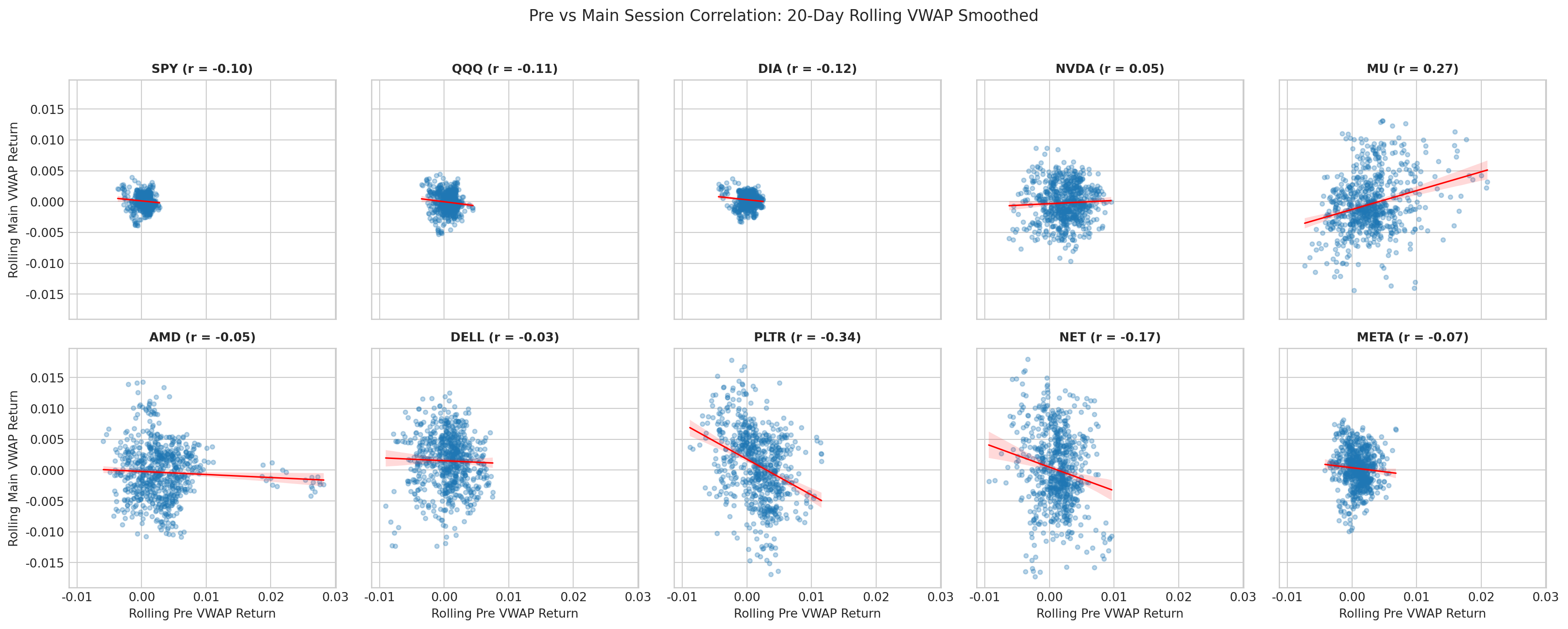
노이즈를 줄이기 위해 세션별 실질 거래량 가중 평균 가격(VWAP)의 \(n\)일 이동평균 및 롤링 누적 수익률을 계산하여 산점도와 상관관계를 비교한다.

Code

SMOOTHING_WINDOW = 20  # 사용자가 쉽게 변경 가능한 스무딩 윈도우 기본값

vwap_corr_list = []
fig, axes = plt.subplots(2, 5, figsize=(18, 7), sharex=True, sharey=True)
axes = axes.flatten()

for i, sym in enumerate(SYMBOLS):
    df_s = df_returns[df_returns['symbol'] == sym].sort_values('trade_date').copy()
    
    # VWAP 기반 롤링 수익률 산출
    df_s['roll_pre_vwap'] = df_s['ret_pre_vwap'].rolling(SMOOTHING_WINDOW).mean()
    df_s['roll_main_vwap'] = df_s['ret_main_vwap'].rolling(SMOOTHING_WINDOW).mean()
    df_s['roll_post_vwap'] = df_s['ret_post_vwap'].rolling(SMOOTHING_WINDOW).mean()
    
    clean = df_s.dropna(subset=['roll_pre_vwap', 'roll_main_vwap'])
    r_val = clean['roll_pre_vwap'].corr(clean['roll_main_vwap'])
    
    vwap_corr_list.append({
        'Symbol': sym,
        'Raw Pre->Main': df_corr_price.loc[sym, 'Pre -> Main'],
        f'VWAP Rolling({SMOOTHING_WINDOW}D) Pre->Main': r_val
    })
    
    # 대표 산점도 시각화: Pre vs Main
    ax = axes[i]
    sns.regplot(data=clean, x='roll_pre_vwap', y='roll_main_vwap', ax=ax,
                scatter_kws={'alpha': 0.3, 's': 12}, line_kws={'color': 'red', 'linewidth': 1.2})
    ax.set_title(f"{sym} (r = {r_val:.2f})", fontsize=10, fontweight='bold')
    ax.set_xlabel('Rolling Pre VWAP Return' if i >= 5 else '')
    ax.set_ylabel('Rolling Main VWAP Return' if i % 5 == 0 else '')

plt.suptitle(f'Pre vs Main Session Correlation: {SMOOTHING_WINDOW}-Day Rolling VWAP Smoothed', fontsize=13, y=1.02)
plt.tight_layout()
plt.show()

pd.DataFrame(vwap_corr_list).set_index('Symbol')

	Raw Pre->Main	VWAP Rolling(20D) Pre->Main
Symbol
SPY	0.018231	-0.096003
QQQ	-0.080771	-0.105074
DIA	-0.036379	-0.115401
NVDA	-0.104767	0.046260
MU	0.010541	0.272408
AMD	-0.045126	-0.053539
DELL	0.034000	-0.033535
PLTR	-0.084024	-0.337440
NET	-0.025334	-0.173973
META	-0.092802	-0.073116

4.4 상위 1% 극단 이벤트 데이 필터링 비교 (Full vs Trimmed)

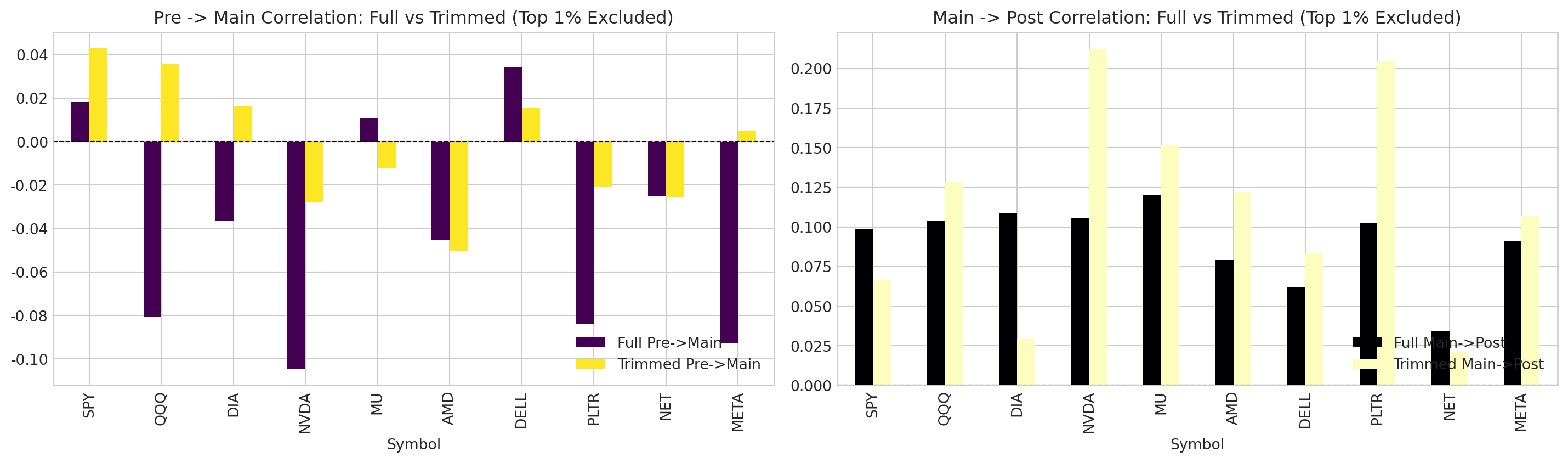
어닝 서프라이즈, FOMC 기준금리 발표일 등 하루 변동성이 상위 1%에 달하는 극단적 이벤트 데이를 제외(Trimmed)했을 때, 평상시 세션 간 선형 상관관계가 어떻게 변모하는지 대조한다.

Code

trimmed_comparison = []

for sym in SYMBOLS:
    df_s = df_returns[df_returns['symbol'] == sym].dropna(subset=['ret_pre_price', 'ret_main_price', 'ret_post_price']).copy()
    
    # 정규장 및 장후 세션 절대 수익률 기준 상위 1% 임계치(99th percentile) 계산
    thresh_main = df_s['ret_main_price'].abs().quantile(0.99)
    thresh_post = df_s['ret_post_price'].abs().quantile(0.99)
    
    # 극단치 제외 (Trimmed)
    df_trimmed = df_s[
        (df_s['ret_main_price'].abs() < thresh_main) & 
        (df_s['ret_post_price'].abs() < thresh_post)
    ]
    
    # 1. Full Dataset
    r_full_pm = df_s['ret_pre_price'].corr(df_s['ret_main_price'])
    r_full_mp = df_s['ret_main_price'].corr(df_s['ret_post_price'])
    
    # 2. Trimmed Dataset
    r_trim_pm = df_trimmed['ret_pre_price'].corr(df_trimmed['ret_main_price'])
    r_trim_mp = df_trimmed['ret_main_price'].corr(df_trimmed['ret_post_price'])
    
    trimmed_comparison.append({
        'Symbol': sym,
        'Full Pre->Main': r_full_pm,
        'Trimmed Pre->Main': r_trim_pm,
        'Diff (Pre->Main)': r_trim_pm - r_full_pm,
        'Full Main->Post': r_full_mp,
        'Trimmed Main->Post': r_trim_mp,
        'Diff (Main->Post)': r_trim_mp - r_full_mp
    })

df_comp = pd.DataFrame(trimmed_comparison).set_index('Symbol')

# 시각화: Full vs Trimmed 상관계수 차이 비교
fig, axes = plt.subplots(1, 2, figsize=(15, 4.5))
df_comp[['Full Pre->Main', 'Trimmed Pre->Main']].plot(kind='bar', ax=axes[0], colormap='viridis')
axes[0].set_title('Pre -> Main Correlation: Full vs Trimmed (Top 1% Excluded)')
axes[0].axhline(0, color='black', linestyle='--', linewidth=0.8)
axes[0].legend(loc='lower right')

df_comp[['Full Main->Post', 'Trimmed Main->Post']].plot(kind='bar', ax=axes[1], colormap='magma')
axes[1].set_title('Main -> Post Correlation: Full vs Trimmed (Top 1% Excluded)')
axes[1].axhline(0, color='black', linestyle='--', linewidth=0.8)
axes[1].legend(loc='lower right')

plt.tight_layout()
plt.show()

df_comp

	Full Pre->Main	Trimmed Pre->Main	Diff (Pre->Main)	Full Main->Post	Trimmed Main->Post	Diff (Main->Post)
Symbol
SPY	0.018231	0.042923	0.024691	0.098907	0.066267	-0.032639
QQQ	-0.080771	0.035440	0.116211	0.104128	0.128521	0.024393
DIA	-0.036379	0.016347	0.052725	0.108516	0.029340	-0.079176
NVDA	-0.104767	-0.028109	0.076659	0.105418	0.212288	0.106870
MU	0.010541	-0.012292	-0.022833	0.120036	0.151715	0.031679
AMD	-0.045126	-0.050231	-0.005105	0.078967	0.121971	0.043005
DELL	0.034000	0.015281	-0.018718	0.061959	0.083529	0.021571
PLTR	-0.084024	-0.021041	0.062983	0.102482	0.204348	0.101866
NET	-0.025334	-0.025664	-0.000330	0.034342	0.020854	-0.013488
META	-0.092802	0.004791	0.097593	0.090844	0.106717	0.015873

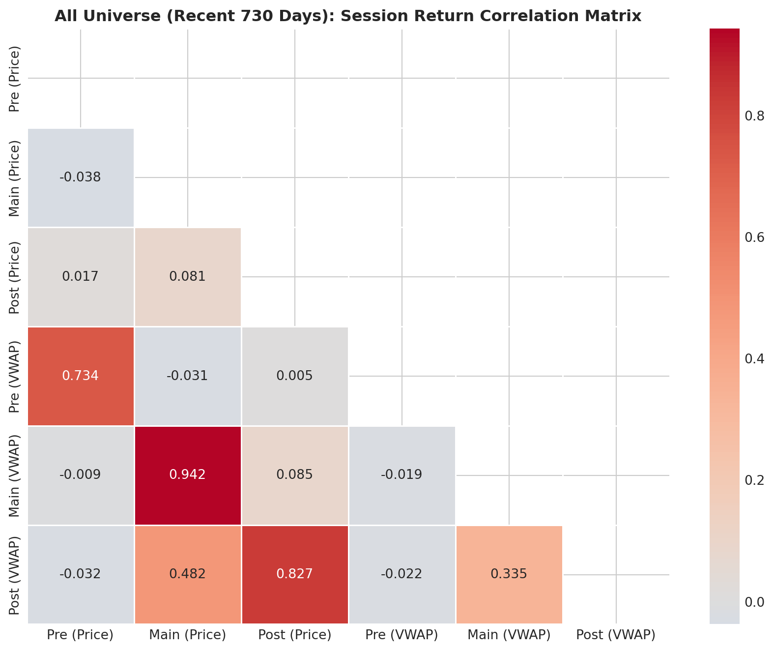
4.5 종합 히트맵 및 자산별 프로파일 비교

Code

# 10개 종목 전체의 세션 수익률 간 피어슨 상관계수 종합 매트릭스
matrix_data = df_returns[[
    'ret_pre_price', 'ret_main_price', 'ret_post_price',
    'ret_pre_vwap', 'ret_main_vwap', 'ret_post_vwap'
]].rename(columns={
    'ret_pre_price': 'Pre (Price)',
    'ret_main_price': 'Main (Price)',
    'ret_post_price': 'Post (Price)',
    'ret_pre_vwap': 'Pre (VWAP)',
    'ret_main_vwap': 'Main (VWAP)',
    'ret_post_vwap': 'Post (VWAP)'
}).corr()

plt.figure(figsize=(9, 7))
mask = np.triu(np.ones_like(matrix_data, dtype=bool))
sns.heatmap(matrix_data, annot=True, fmt='.3f', cmap='coolwarm', center=0, mask=mask, linewidths=0.5)
plt.title('All Universe (Recent 730 Days): Session Return Correlation Matrix', fontsize=12, fontweight='bold')
plt.tight_layout()
plt.show()

1 서론

1.1 분석 가설

2 분석 대상

3 데이터 수집

3.1 데이터 수집 환경 및 사전 준비

3.2 세션별 시점 및 수익률 정의

3.2.1 단순 가격(Close) 기반 수익률

3.2.2 세션별 VWAP (Volume-Weighted Average Price) 산출

3.3 데이터 파이프라인 및 Parquet 캐싱

4 방법론 및 결과 분석

4.1 세션별 지표 집계 및 DuckDB 가공 (session_features)

4.2 단순 가격 일간 수익률 간 선형 상관관계 (Baseline Correlation)

4.3 세션별 VWAP 롤링 스무딩 상관관계 (VWAP Smoothed Correlation, \(n=20\))

4.4 상위 1% 극단 이벤트 데이 필터링 비교 (Full vs Trimmed)

4.5 종합 히트맵 및 자산별 프로파일 비교

4.1 세션별 지표 집계 및 DuckDB 가공 (`session_features`)