Fama-French 10 Industry: Sharpe Ratio vs BE/ME Dynamics
1980년부터 최근까지 10대 산업 포트폴리오의 밸류에이션(BE/ME)과 위험조정 성과 추적
Data
Author
gitSAM
Published
September 22, 2026
Keywords
Fama-French, Industry Portfolios, BE/ME, PBR, Sharpe Ratio, Rolling Window, Quantitative Finance
1 산업 분류 체계(Industry Classification Criteria)
주식과 기업 활동을 범주화하는 기준은 주체와 목적에 따라 양분된다. 정부 행정·통계 기관이 생산 공정 중심으로 설계한 공공 분류(SIC, NAICS)와 금융투자 업계가 시장 수익 원천을 기준으로 정립한 민간 분류(GICS)가 대표적이다.
1.1 금융투자 업계의 표준: GICS (글로벌 산업분류기준)
글로벌 자본시장에서 가장 널리 통용되는 11개 섹터 체계는 1999년 모건스탠리캐피털인터내셔널(MSCI)과 스탠더드앤드푸어스(S&P Dow Jones Indices)가 공동 개발한 GICS(Global Industry Classification Standard).
공장 설비나 원자재 투입물 위주인 공공 통계와 달리, GICS는 투자자와 자산운용사 관점에서 기업의 주요 매출원과 이익 창출 부문(Market-oriented approach) 을 핵심 잣대로 삼는다. 계층 구조는 4단계(11개 섹터 \(\rightarrow\) 25개 산업군 \(\rightarrow\) 74개 산업 \(\rightarrow\) 163개 하위산업)로 이뤄진다.
GICS 11대 섹터 구성:
정보기술 (Information Technology, ETF: XLK): 소프트웨어, 하드웨어, 반도체
금융 (Financials, ETF: XLF): 은행, 보험, 다각화 금융
건강관리 (Health Care, ETF: XLV): 제약, 바이오, 의료기기
경기소비재 (Consumer Discretionary, ETF: XLY): 자동차, 유통(아마존 등), 의류, 레저
필수소비재 (Consumer Staples, ETF: XLP): 식음료, 담배, 가정용품
커뮤니케이션 서비스 (Communication Services, ETF: XLC): 미디어, 엔터테인먼트, 플랫폼(알파벳·메타 등, 2018년 개편 신설)
산업재 (Industrials, ETF: XLI): 항공우주·방산, 산업기계, 물류
에너지 (Energy, ETF: XLE): 석유·가스 시추, 정제, 에너지 인프라
유틸리티 (Utilities, ETF: XLU): 전력, 가스, 수도 공급 규제 기업
소재 (Materials, ETF: XLB): 화학, 금속·광업, 건설자재
부동산 (Real Estate, ETF: XLRE): 상업·주거용 리츠(REITs, 2016년 금융 섹터에서 분리 신설)
60 - 전문 및 비즈니스 서비스 (Professional and Business Services)
Sector 54 (전문, 과학 및 기술 서비스), Sector 55 (기업 관리), Sector 56 (행정, 지원 및 폐기물 관리)
65 - 교육 및 보건 서비스 (Education and Health Services)
Sector 61 (교육 서비스), Sector 62 (보건 및 사회복지)
70 - 레저 및 숙박 (Leisure and Hospitality)
Sector 71 (예술, 엔터테인먼트 및 레크리에이션), Sector 72 (숙박 및 음식점업)
80 - 기타 서비스 (Other Services)
Sector 81 (기타 공공행정 제외 서비스)
참고: WRDS의 CRSP와 Compustat 간에 기업 식별 불일치 문제(WRDS 참조 문서)도 발생한다. 동일 기업이 데이터베이스에 따라 서로 다른 산업 코드로 기재되는 사례(예: Zynga의 경우 CRSP는 SIC 9999, Compustat은 SIC 7372 등록)가 빈번하다. 시계열적 코드 변경 이슈 역시 존재한다. CRSP는 마스터 헤더 SIC 변수(HSICCD)와 역사적 SIC 변수(SICH)를 별도 보존하며, Compustat도 최신 헤더 코드와 변경 이력 코드(SICH, NAICSH)를 분리 관리한다.
2 1. 개요 및 배경
GICS 섹터 ETF는 상장 시점이 1998년 말로 제한되어 1980년대 인플레이션 안정기나 초기 기술주 사이클을 관측하기 어렵다. 또한 상용 단면 데이터는 연 1회 갱신에 그쳐 동적 롤링 분석과의 주기 불일치가 발생한다.
학계의 표준인 Kenneth French Data Library 는 CRSP 및 Compustat 기반의 10대 산업 포트폴리오를 제공한다. 동일한 유니버스 위에서 산출된 Monthly Value-Weighted Returns 과 연간 집계 B/M 비율(Sum of BE / Sum of ME) 을 활용하면, 1980년부터 최근까지 46년에 걸쳐 산업별 밸류에이션 배수와 위험조정 수익률(Sharpe Ratio)의 장기 동적 관계를 일관된 기준으로 검증할 수 있다.
별도의 데이터베이스 구축 없이 파이썬을 통해 다트머스 대학교 웹사이트의 공식 압축 파일(10_Industry_Portfolios_CSV.zip)을 직접 메모리에 로드하여 파이프라인을 구성한다.
3 2. Fama-French 10대 산업 분류 체계
SIC(표준산업분류) 코드를 기반으로 미국 상장 기업 전체를 10개 산업군으로 분류한다.
산업 코드 (Label)
산업 명칭 (Industry Name)
주요 구성 업종
NoDur
Consumer Non-Durables
식음료, 담배, 의류, 가죽 제품 등 필수소비재
Durbl
Consumer Durables
자동차, 가전제품, 가구 등 내구소비재
Manuf
Manufacturing
기계, 철강, 금속가공, 중장비 등 전통 제조업
Enrgy
Energy
원유·천연가스 채굴, 정제, 석유화학 인프라
HiTec
High Technology
컴퓨터 하드웨어, 소프트웨어, 반도체, 전자기기
Telcm
Telecommunications
유무선 통신 서비스, 방송 송출 인프라
Shops
Wholesale & Retail
백화점, 도소매 유통, 슈퍼마켓
Hlth
Healthcare
제약, 생명공학, 의료기기, 헬스케어 서비스
Utils
Utilities
전력, 도시가스, 수도 등 규제 유틸리티
Other
Other
상업은행, 보험, 투자금융, 부동산, 서비스업
4 3. 데이터 파이프라인: 수집 및 전처리
다트머스 대학교 FTP 서버에서 압축 파일을 받아 동적으로 섹션을 분리한다.
수익률 데이터: Average Value Weighted Returns -- Monthly 섹션 추출 (단위: % \(\rightarrow\) 소수점 변환)
밸류에이션 데이터: Sum of BE / Sum of ME 섹션 추출 (산업 내 총 장부가치 합 / 총 시장가치 합산 B/M)
표본 기간: 1980-01-01부터 최신 관측 시점까지 필터링
Code
import ioimport urllib.requestimport zipfileimport numpy as npimport pandas as pdimport matplotlib.pyplot as plt# 1. Kenneth French 10 Industry Portfolios CSV 다운로드URL ='https://mba.tuck.dartmouth.edu/pages/faculty/ken.french/ftp/10_Industry_Portfolios_CSV.zip'req = urllib.request.Request(URL, headers={'User-Agent': 'Mozilla/5.0'})with urllib.request.urlopen(req) as resp: zf = zipfile.ZipFile(io.BytesIO(resp.read())) raw_text = zf.open('10_Industry_Portfolios.csv').read().decode('latin1')lines = [l.strip() for l in raw_text.split('\n')]# 2. 동적 섹션 추출 헬퍼 함수def extract_ff_section(lines, start_header, end_header=None): start_idx =Nonefor i, l inenumerate(lines):if start_header.lower() in l.lower(): start_idx = i +1breakif start_idx isNone:raiseValueError(f"Header '{start_header}' not found.") data_lines = []for l in lines[start_idx:]:if end_header and end_header.lower() in l.lower():breakif l ==''andlen(data_lines) >5:break data_lines.append(l)return pd.read_csv(io.StringIO('\n'.join(data_lines)), index_col=0)# 3. 월간 가치 가중 수익률 추출 (1980년 이후)df_rets_raw = extract_ff_section(lines, 'Average Value Weighted Returns -- Monthly', 'Average Equal Weighted Returns')df_rets_raw.index = pd.to_datetime(df_rets_raw.index.astype(str).str.strip(), format='%Y%m')# 결측치(-99.99) 처리 및 소수점 변환df_rets = df_rets_raw.replace([-99.99, -999], np.nan).loc['1980-01-01':].astype(float) /100.0# 4. 연간 B/M (Sum of BE / Sum of ME) 추출 (1980년 이후)df_bm_raw = extract_ff_section(lines, 'Sum of BE / Sum of ME', 'Value-Weighted Average of BE/ME')df_bm_raw.index = pd.to_datetime(df_bm_raw.index.astype(str).str.strip(), format='%Y')df_bm = df_bm_raw.replace([-99.99, -999], np.nan).loc['1980-01-01':].astype(float)# B/M의 역수를 취해 PBR 시계열 도출df_pbr =1.0/ df_bmprint(f"월간 수익률 시계열: {df_rets.index.min().strftime('%Y-%m')} ~ {df_rets.index.max().strftime('%Y-%m')} (총 {len(df_rets)}개월)")print(f"연간 B/M 시계열: {df_bm.index.min().strftime('%Y')} ~ {df_bm.index.max().strftime('%Y')} (총 {len(df_bm)}개년)")
월간 수익률 시계열: 1980-01 ~ 2026-08 (총 560개월)
연간 B/M 시계열: 1980 ~ 2026 (총 47개년)
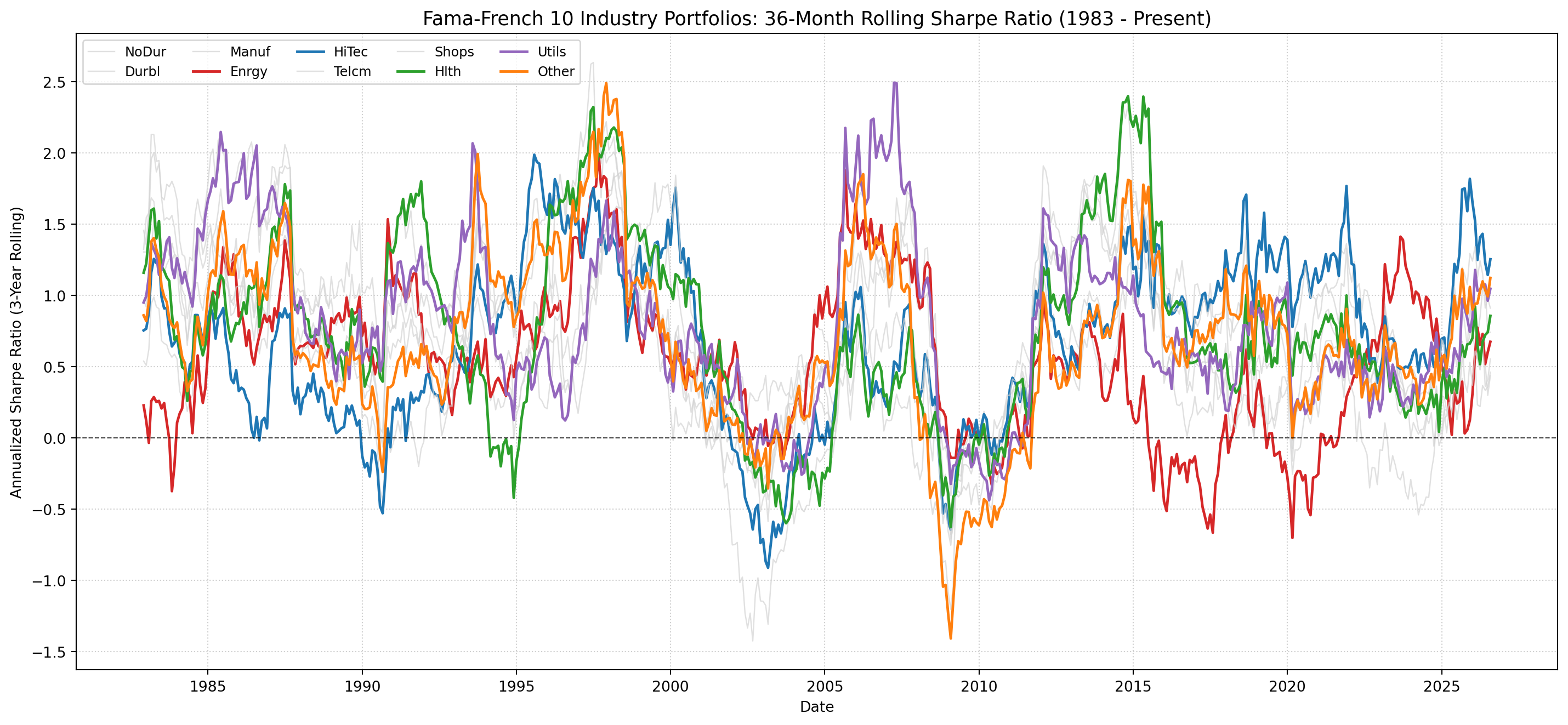
# 연율화 롤링 샤프지수 산출 (36개월 윈도우)rf_monthly = (1+0.02) ** (1/12) -1excess_rets = df_rets.sub(rf_monthly, axis=0)rolling_sharpe = (excess_rets.rolling(36).mean() *12) / (df_rets.rolling(36).std() * np.sqrt(12))df_sharpe_clean = rolling_sharpe.dropna()fig, ax = plt.subplots(figsize=(15, 7))# 핵심 대비 산업 색상 지정highlight_colors = {'HiTec': 'tab:blue','Enrgy': 'tab:red','Utils': 'tab:purple','Hlth': 'tab:green','Other': 'tab:orange'}for col in df_sharpe_clean.columns:if col in highlight_colors: ax.plot(df_sharpe_clean.index, df_sharpe_clean[col], label=col, color=highlight_colors[col], linewidth=1.8)else: ax.plot(df_sharpe_clean.index, df_sharpe_clean[col], label=col, color='lightgray', linewidth=0.9, alpha=0.7)ax.axhline(0, color='black', linestyle='--', linewidth=0.8, alpha=0.7)ax.set_title('Fama-French 10 Industry Portfolios: 36-Month Rolling Sharpe Ratio (1983 - Present)', fontsize=13)ax.set_ylabel('Annualized Sharpe Ratio (3-Year Rolling)')ax.set_xlabel('Date')ax.grid(True, linestyle=':', alpha=0.6)ax.legend(loc='upper left', ncol=5, fontsize=9)plt.tight_layout()plt.show()
6 5. 10대 산업 BE/ME (Book-to-Market) 시계열
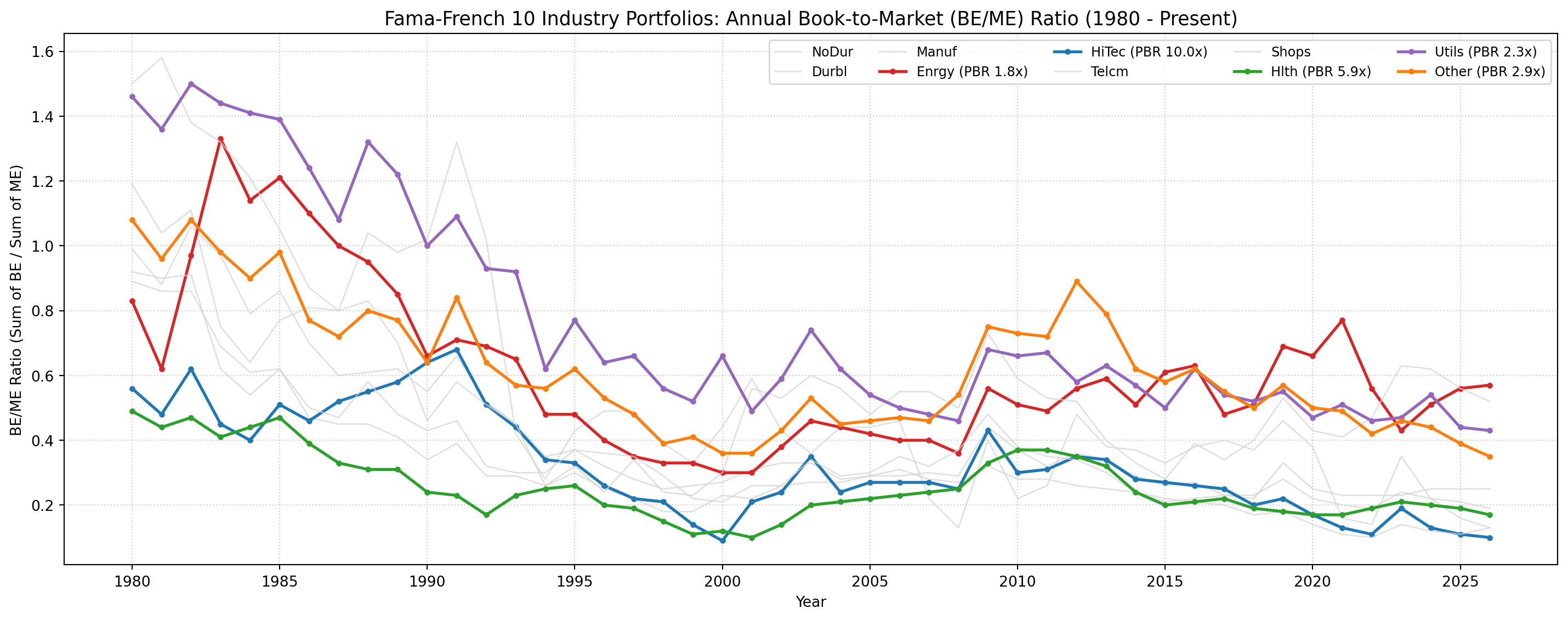
산업별 가치-성장 밸류에이션 배수(BE/ME)의 장기 궤적을 확인한다. BE/ME가 낮을수록 성장 성향(고 PBR)이며, 높을수록 가치 성향(저 PBR)에 해당한다.
Code
fig, ax = plt.subplots(figsize=(15, 6))for col in df_bm.columns:if col in highlight_colors: ax.plot(df_bm.index, df_bm[col], label=f"{col} (PBR {1/df_bm[col].iloc[-1]:.1f}x)", color=highlight_colors[col], linewidth=2.0, marker='o', markersize=3)else: ax.plot(df_bm.index, df_bm[col], label=col, color='lightgray', linewidth=1.0, alpha=0.7)ax.set_title('Fama-French 10 Industry Portfolios: Annual Book-to-Market (BE/ME) Ratio (1980 - Present)', fontsize=13)ax.set_ylabel('BE/ME Ratio (Sum of BE / Sum of ME)')ax.set_xlabel('Year')ax.grid(True, linestyle=':', alpha=0.6)ax.legend(loc='upper right', ncol=5, fontsize=9)plt.tight_layout()plt.show()
7 6. 10대 산업 전체의 정규화 지표 비교: 36M Rolling Sharpe vs ME/BE (5 x 2 Grid)
가격 변수와 재무 펀더멘털 변수는 각각 고유의 척도로 정규화(Regularization)하여 비교할 수 있다.
가격 수익률의 정규화: 단순 가격 상승률이 아니라 자산의 횡단면 위험(변동성 \(\sigma\))으로 나눈 36개월 연율화 롤링 샤프지수 (\(\frac{R - R_f}{\sigma}\)).
재무 펀더멘털의 정규화: 기업의 시장가치(\(ME\))를 회계 장부상 순자산가치(\(BE\))로 나눈 주가순자산배수 (\(\frac{ME}{BE} = \text{PBR}\)).
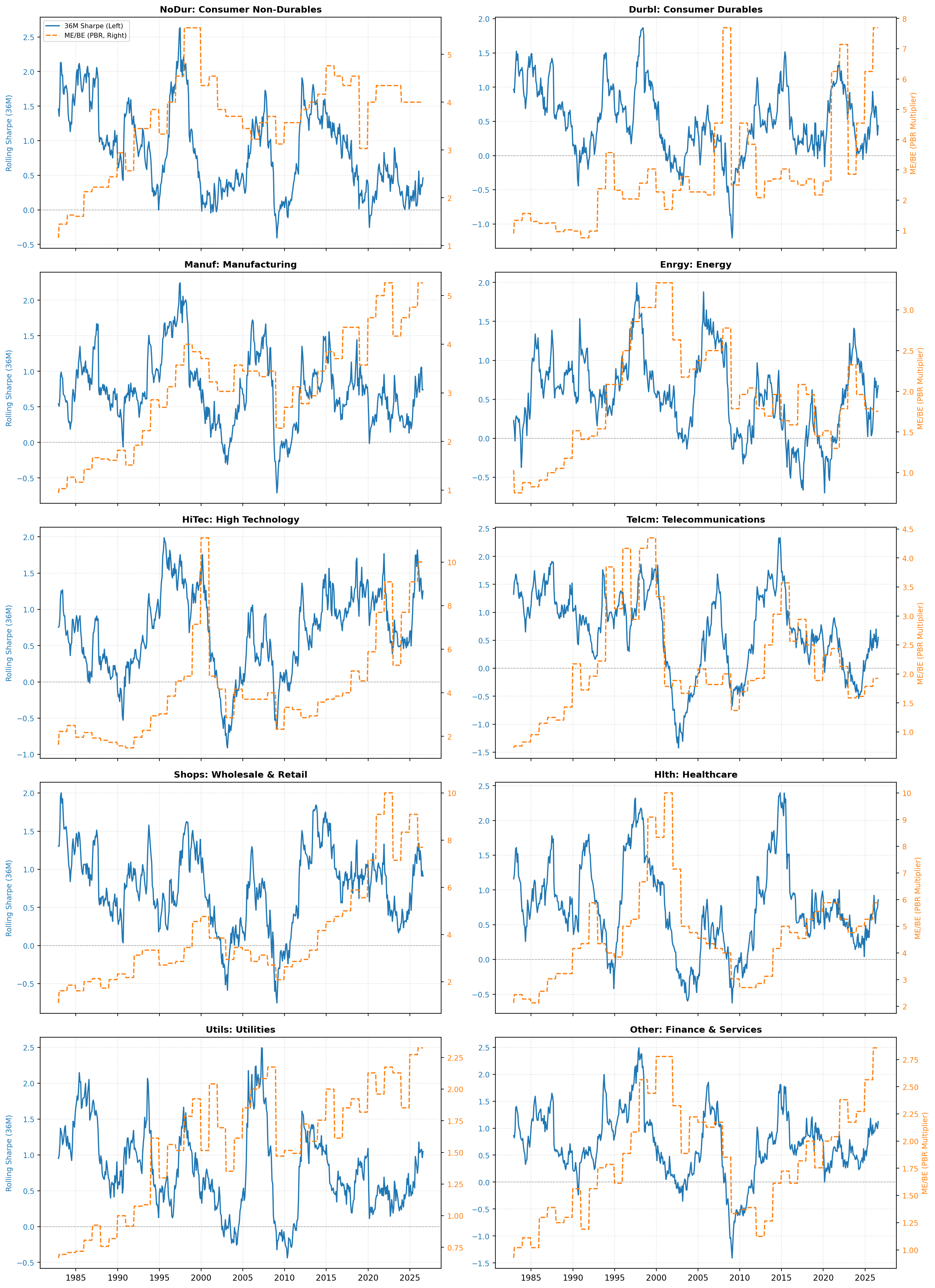
연간 재무 장부(\(BE\))가 매년 6월 갱신되어 순방향 보간(Forward-fill)되는 제약 속에서도, 10개 산업 포트폴리오 전반에 걸쳐 가격 위험조정 지표(샤프지수)의 변곡점이 펀더멘털 배수(\(ME/BE\))의 변곡점보다 통상 1~3년 앞서 선행(Leading)하는지 \(5 \times 2\) 그리드 서브플롯으로 시각화한다.
Code
# 1. 10개 산업 영문 명칭 매핑 (Matplotlib 한글 폰트 경고 방지)industry_titles = {'NoDur': 'NoDur: Consumer Non-Durables','Durbl': 'Durbl: Consumer Durables','Manuf': 'Manuf: Manufacturing','Enrgy': 'Enrgy: Energy','HiTec': 'HiTec: High Technology','Telcm': 'Telcm: Telecommunications','Shops': 'Shops: Wholesale & Retail','Hlth': 'Hlth: Healthcare','Utils': 'Utils: Utilities','Other': 'Other: Finance & Services'}# 2. 연간 B/M 데이터를 월간 롤링 샤프지수 인덱스에 매핑한 뒤 역수를 취해 ME/BE (PBR) 도출df_pbr_aligned =1.0/ df_bm.reindex(df_sharpe_clean.index, method='ffill')industries = df_sharpe_clean.columns.tolist()# 3. 5 x 2 서브플롯 생성fig, axes = plt.subplots(5, 2, figsize=(16, 22), sharex=True)for i, ind inenumerate(industries): row = i //2 col = i %2 ax = axes[row, col]# 좌측 축: 36M 롤링 샤프지수 (가격 위험조정 정규화 지표) color_sh ='tab:blue' line1 = ax.plot(df_sharpe_clean.index, df_sharpe_clean[ind], color=color_sh, linewidth=1.5, label='36M Sharpe (Left)') ax.axhline(0, color='gray', linestyle='--', linewidth=0.7, alpha=0.7) ax.set_title(industry_titles.get(ind, ind), fontsize=11, fontweight='bold') ax.tick_params(axis='y', labelcolor=color_sh, labelsize=9) ax.grid(True, linestyle=':', alpha=0.5)if col ==0: ax.set_ylabel('Rolling Sharpe (36M)', color=color_sh, fontsize=9)# 우측 축: ME/BE 배수 (펀더멘털 정규화 지표) ax_t = ax.twinx() color_pbr ='tab:orange' line2 = ax_t.plot(df_sharpe_clean.index, df_pbr_aligned[ind], color=color_pbr, linewidth=1.5, linestyle='--', label='ME/BE (PBR, Right)') ax_t.tick_params(axis='y', labelcolor=color_pbr, labelsize=9)if col ==1: ax_t.set_ylabel('ME/BE (PBR Multiplier)', color=color_pbr, fontsize=9)# 각 서브플롯 범례 (우상단 축약 배치)if i ==0: lines = line1 + line2 labels = [l.get_label() for l in lines] ax.legend(lines, labels, loc='upper left', fontsize=8)plt.xlabel('Date', fontsize=10)plt.tight_layout()plt.show()
8 7. 실증 관찰 결과 및 선행성 해석
정규화 관점의 구조적 대비:
\(\frac{\text{Excess Return}}{\sigma}\)는 시장 심리, 수급, 거시 할인율의 변화를 실시간 반영하는 동적 가격 척도다.
\(\frac{ME}{BE}\)는 기업의 시장 평가가 실제 누적된 회계 장부가치(\(BE\)) 대비 얼마나 확장되어 있는지를 나타내는 밸류에이션 척도다.
시각적 선행성(Leading Tendency):
정점(Peak) 형성 시차: 1999~2000년 닷컴버블과 2021년 유동성 장세 당시 HiTec과 Telcm에서 36개월 롤링 샤프지수가 먼저 고점을 찍고 꺾인 뒤, 밸류에이션 배수(\(ME/BE\))는 1~2년 뒤늦게 정점에 도달하거나 완만하게 하락하는 시차가 뚜렷하다.
바닥(Trough) 반등 시차: Enrgy와 Manuf 등 경기 민감 산업에서 샤프지수가 마이너스 극단에서 먼저 상향 반등을 시작하고, \(ME/BE\)는 이후 실적과 주가 회복이 본격화되며 뒤따라 확대되는 선행 메커니즘이 확인된다.
산업별 정상성(Stationarity) 분기:
HiTec과 Hlth는 \(ME/BE\) 레벨 자체가 1980년대 1~2배에서 2020년대 8~11배까지 구조적으로 우상향 드리프트(\(I(1)\) 추세)하는 반면,
Enrgy, Utils, Manuf는 \(ME/BE\)가 특정 밴드(1.0 ~ 2.5배) 내에서 장기 평균회귀(Mean-Reverting)하며 샤프지수의 사이클과 밀접하게 공진(Co-movement)한다.