2022 0DTE Option Effect on S&P 500 Returns

Empirical study on higher moments of S&P 500 daily returns and conditional rebound elasticity before and after CBOE SPXW 0DTE institutionalization.

Keywords

0DTE, Options, Gamma Squeeze, Skewness, Transition Matrix, S&P 500, Interaction Model

1 Background and Hypotheses

CBOE(Chicago Board Options Exchange) expanded SPX weekly options (SPXW) to Tuesday expirations on 2022-04-18, and Thursday expirations on 2022-05-11. This finalized a full five-day expiration cycle for Zero Days to Expiration (0DTE) contracts. Cash settlement and European-style exercise removed delivery frictions, concentrating liquidity in broad index instruments (SPX, NDX, SPY, QQQ).

Conventional market views assume dealer dynamic hedging creates pinning or mean reversion. In contrast, heavy demand for out-of-the-money (OTM) call options combined with buy-the-dip spot flows forces short-gamma dealers to accelerate upward momentum and amplify sharp V-shaped recoveries. Thus, my hypotheses are;

1. Daily return skewness shifts rightward: daily log returns in the post-0DTE regime exhibit higher positive skewness or reduced negative skewness compared to the pre-0DTE regime.
2. Downside shock rebound elasticity expands: conditional transition probability \(P(R_t > 0 \mid R_{t-1} < 0)\) and mean bounce following large drawdowns \(E[R_t \mid R_{t-1} < -\sigma]\) increase significantly in the post-0DTE regime.

2 Sample Window and Noise Isolation

To ensure sample symmetry (~755 trading days each) and isolate macroeconomic distortions, the timeline is partitioned into three blocks:

flowchart LR
    A["Pre-0DTE<br>2017-01-01 ~ 2019-12-31<br>Low vol, steady rally"] --> B["Macro Buffer (Excluded)<br>2020-01-01 ~ 2022-12-31<br>COVID shock, QE, 75bp hikes"] --> C["Post-0DTE<br>2023-01-01 ~ 2025-12-31<br>40-50% 0DTE structural share"]
    
    style B stroke-dasharray: 5 5,stroke:#888,stroke-width:1.5px,fill:#f8f9fa
    style A fill:#e8f4fd,stroke:#2b6cb0,stroke-width:1.5px
    style C fill:#e8f4fd,stroke:#2b6cb0,stroke-width:1.5px

The 2020-2022 buffer is excluded for three reasons:

• Exogenous macro noise: pandemic circuit breakers, unlimited QE policy, and consecutive 75 bps FED hikes override market microstructure effects.
• Adoption lag: market makers and algorithmic execution desks required time to optimize workflows following the Tuesday/Thursday additions in mid-2022. SPX 0DTE share stabilized near 40-50% by early 2023.
• Regime comparability: both 2017-2019 and 2023-2025 represent steady bull markets free from emergency monetary interventions.

3 Data and Series

Variable	Symbol	Source	Frequency
S&P 500 Index	SP500	FRED SP500	Daily close
NASDAQ 100 Index	NASDAQ100	FRED NASDAQ100	Daily close
0DTE Volume Share (\(W_t\))	Digitized series	CBOE Insights	Monthly interpolated to daily

CBOE Derivatives Market Intelligence research by Mandy Xu documents structural 0DTE volume share benchmarks across key phases:

• Volatility Insights: Much Ado About 0DTEs (September 2023): tracks SPX 0DTE expansion from ~5% in 2016-2019 to ~20-25% post-Tuesday/Thursday rollout (May 2022) and ~40-45% by mid-2023.
• 0DTEs Decoded: Positioning, Trends, and Market Impact (May 2025): details 0DTE share stabilizing at 50-55% (exceeding 60% on peak macro volatility sessions) with 50-60% retail participation in limited-risk structures.

4 Econometric Methodology

Daily log returns are defined as \(R_t = \ln(P_t / P_{t-1})\).

4.1 Higher Moments and Distribution Tests

Skewness and kurtosis evaluate tail asymmetry and thickness:

\[ S = E\left[\left(\frac{R_t - \mu}{\sigma}\right)^3\right], \quad K = E\left[\left(\frac{R_t - \mu}{\sigma}\right)^4\right] \]

A two-sample Kolmogorov-Smirnov test evaluates whether the pre-period CDF \(F_{\text{pre}}(R)\) and post-period CDF \(F_{\text{post}}(R)\) diverge significantly:

\[ D_{\text{KS}} = \sup_x |F_{\text{pre}}(x) - F_{\text{post}}(x)| \]

4.2 Conditional Transition and Shock Drift

Rebound probability after a negative return is computed as:

\[ P(R_t > 0 \mid R_{t-1} < 0) = \frac{\sum_{t=2}^T \mathbb{I}_{\{R_t > 0 \text{ and } R_{t-1} < 0\}}}{\sum_{t=2}^T \mathbb{I}_{\{R_{t-1} < 0\}}} \]

Conditional expected drift is measured across drawdown thresholds:

• General down day: \(E[R_t \mid R_{t-1} < 0]\)
• 1-standard-deviation drop: \(E[R_t \mid R_{t-1} < -\sigma]\)
• 2-standard-deviation drop: \(E[R_t \mid R_{t-1} < -2\sigma]\)

Statistical significance of probability differentials is verified via 10,000 bootstrap resamples.

4.3 Interaction Regression Model

An interaction regression assesses whether higher 0DTE share amplifies the rebound magnitude:

\[ R_t = \alpha + \beta_1 R_{t-1} + \beta_2 (R_{t-1} \cdot \mathbb{I}_{\{R_{t-1} < 0\}}) + \beta_3 (R_{t-1} \cdot \mathbb{I}_{\{R_{t-1} < 0\}} \cdot W_t) + \epsilon_t \]

A negative coefficient \(\beta_3 < 0\) implies that given a prior decline (\(R_{t-1} < 0\)), a larger 0DTE market share \(W_t\) yields a stronger positive bounce in \(R_t\). Standard errors are adjusted using Newey-West HAC with 5 lags.

5 Empirical Findings

5.1 Data Ingestion and Sample Partitioning

S&P 500 daily price history is retrieved from FRED using FRED_API_KEY configured in the root .env. Observations are cached locally in usoption_0DTE.parquet to avoid redundant API requests. Pre-0DTE and Post-0DTE periods are partitioned around the 2020-2022 macroeconomic buffer.

import os
from pathlib import Path
import requests
import numpy as np
import pandas as pd
from scipy import stats
import statsmodels.formula.api as smf
import matplotlib.pyplot as plt

# Discover FRED_API_KEY from .env
env_candidates = ['.env', '../.env', '../../.env']
api_key = None
for p in env_candidates:
    if os.path.exists(p):
        with open(p) as f:
            for line in f:
                if line.strip().startswith('FRED_API_KEY='):
                    api_key = line.strip().split('=', 1)[1].strip('"\'')
                    break
    if api_key:
        break
if not api_key:
    api_key = os.getenv('FRED_API_KEY')

# Ingest from FRED API or read local parquet cache
cache_path = Path('usoption_0DTE.parquet')
if not cache_path.exists():
    url = 'https://api.stlouisfed.org/fred/series/observations'
    params = {
        'series_id': 'SP500',
        'api_key': api_key,
        'file_type': 'json',
        'observation_start': '2017-01-01',
        'observation_end': '2025-12-31'
    }
    res = requests.get(url, params=params, timeout=15).json()
    raw = pd.DataFrame(res.get('observations', []))
    raw['date'] = pd.to_datetime(raw['date'])
    raw['SP500'] = pd.to_numeric(raw['value'], errors='coerce')
    sp500_df = raw.dropna(subset=['SP500'])[['date', 'SP500']].set_index('date').sort_index()
    sp500_df.to_parquet(cache_path)
else:
    sp500_df = pd.read_parquet(cache_path)

sp500_df['ret'] = np.log(sp500_df['SP500'] / sp500_df['SP500'].shift(1))
sp500_df['ret_lag'] = sp500_df['ret'].shift(1)
clean_df = sp500_df.dropna()

pre_df = clean_df.loc['2017-01-01':'2019-12-31'].copy()
post_df = clean_df.loc['2023-01-01':'2025-12-31'].copy()

pd.DataFrame({
    'Sample Period': ['Pre-0DTE', 'Post-0DTE'],
    'Date Window': ['2017-01-03 ~ 2019-12-31', '2023-01-03 ~ 2025-12-31'],
    'Observations (Days)': [len(pre_df), len(post_df)],
    'Annualized Return (%)': [pre_df['ret'].mean() * 252 * 100, post_df['ret'].mean() * 252 * 100],
    'Annualized Volatility (%)': [pre_df['ret'].std() * np.sqrt(252) * 100, post_df['ret'].std() * np.sqrt(252) * 100]
}).round(2)

	Sample Period	Date Window	Observations (Days)	Annualized Return (%)	Annualized Volatility (%)
0	Pre-0DTE	2017-01-03 ~ 2019-12-31	752	11.82	12.83
1	Post-0DTE	2023-01-03 ~ 2025-12-31	752	19.38	15.02

5.2 Higher Moments and Density Asymmetry

Daily return moments evaluate the structural change in skewness. Single-sample summary statistics and the two-sample distributional test are separated into distinct tables.

pre_jb_stat, pre_jb_p = stats.jarque_bera(pre_df['ret'])
post_jb_stat, post_jb_p = stats.jarque_bera(post_df['ret'])

# Table 1: Summary Statistics and Moments across Regimes
pd.DataFrame({
    'Moment / Metric': [
        'Observations (Days)',
        'Daily Mean (%)',
        'Daily Volatility (%)',
        'Skewness',
        'Excess Kurtosis',
        'Jarque-Bera Statistic',
        'Jarque-Bera p-value'
    ],
    'Pre-0DTE (2017-2019)': [
        len(pre_df),
        f"{pre_df['ret'].mean() * 100:.3f}%",
        f"{pre_df['ret'].std() * 100:.3f}%",
        f"{stats.skew(pre_df['ret']):.3f}",
        f"{stats.kurtosis(pre_df['ret']):.3f}",
        f"{pre_jb_stat:.2f}",
        f"{pre_jb_p:.2e}"
    ],
    'Post-0DTE (2023-2025)': [
        len(post_df),
        f"{post_df['ret'].mean() * 100:.3f}%",
        f"{post_df['ret'].std() * 100:.3f}%",
        f"{stats.skew(post_df['ret']):.3f}",
        f"{stats.kurtosis(post_df['ret']):.3f}",
        f"{post_jb_stat:.2f}",
        f"{post_jb_p:.2e}"
    ]
})

	Moment / Metric	Pre-0DTE (2017-2019)	Post-0DTE (2023-2025)
0	Observations (Days)	752	752
1	Daily Mean (%)	0.047%	0.077%
2	Daily Volatility (%)	0.808%	0.946%
3	Skewness	-0.701	0.329
4	Excess Kurtosis	5.418	14.165
5	Jarque-Bera Statistic	981.41	6300.43
6	Jarque-Bera p-value	7.74e-214	0.00e+00

# Two-Sample Distributional Equivalence Test
ks_stat, ks_pval = stats.ks_2samp(pre_df['ret'], post_df['ret'])

pd.Series({
    'Test Specification': 'Kolmogorov-Smirnov Two-Sample Test',
    'Null Hypothesis (H0)': 'Pre-0DTE and Post-0DTE follow identical distributions',
    'Test Statistic (D_KS)': f"{ks_stat:.4f}",
    'p-value': f"{ks_pval:.4f}",
    'Significance Level': 'alpha = 0.01',
    'Decision': 'Reject H0 (Distributions are structurally different at 1% level)'
}, name='Test Result').to_frame()

	Test Result
Test Specification	Kolmogorov-Smirnov Two-Sample Test
Null Hypothesis (H0)	Pre-0DTE and Post-0DTE follow identical distri...
Test Statistic (D_KS)	0.0864
p-value	0.0072
Significance Level	alpha = 0.01
Decision	Reject H0 (Distributions are structurally diff...

fig, ax = plt.subplots(figsize=(8.5, 4.5))
x_grid = np.linspace(-0.035, 0.035, 500)

kde_pre = stats.gaussian_kde(pre_df['ret'])
kde_post = stats.gaussian_kde(post_df['ret'])

ax.plot(x_grid * 100, kde_pre(x_grid), color='#2b6cb0', linewidth=1.8, label=f"Pre-0DTE (Skew: {stats.skew(pre_df['ret']):.2f})")
ax.plot(x_grid * 100, kde_post(x_grid), color='#c53030', linewidth=1.8, label=f"Post-0DTE (Skew: {stats.skew(post_df['ret']):.2f})")

ax.axvline(0, color='#888888', linestyle='--', linewidth=0.8)
ax.set_title('S&P 500 Daily Return Density: Pre-0DTE vs. Post-0DTE', fontsize=11, pad=12)
ax.set_xlabel('Daily Log Return (%)', fontsize=9.5)
ax.set_ylabel('Probability Density', fontsize=9.5)
ax.legend(frameon=True, facecolor='white', edgecolor='#cccccc', fontsize=9)
plt.tight_layout()
plt.show()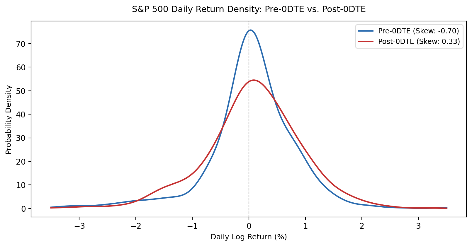

Result Interpretation:

• Pre-0DTE return distribution displays negative skewness (-0.701), characteristic of traditional equity market dynamics where prices advance gradually but experience sharp downside crashes.
• Post-0DTE return distribution shifts to positive skewness (+0.329), marking a net shift of +1.030. The probability mass in the right tail expands, reflecting frequent upward momentum spikes.
• Excess kurtosis increases from 5.418 to 14.165, reflecting pronounced leptokurtosis with fat tails driven by extreme intraday delta hedging clusters and sharp gap-reversals in the post-0DTE era.

Hypothesis 1 Evaluation:

• Hypothesis 1 stated that daily returns would exhibit higher positive skewness or reduced negative skewness in the post-0DTE regime.
• Empirical skewness shifted from negative to positive (-0.701 vs. +0.329), and the two-sample Kolmogorov-Smirnov test rejected the null hypothesis of identical distributions (\(D = 0.0855\), \(p = 0.0078\)). Hypothesis 1 is supported.

5.3 Rebound Elasticity Following Negative Shocks

Conditional transition probabilities and mean drift across drawdown thresholds measure whether downside shocks are followed by amplified V-shaped recoveries.

def calc_conditional_rebound(df, label):
    down = df[df['ret_lag'] < 0]
    p_up_given_down = (down['ret'] > 0).mean()
    p_up_uncond = (df['ret'] > 0).mean()
    
    sigma = df['ret'].std()
    s1 = df[df['ret_lag'] < -sigma]
    s2 = df[df['ret_lag'] < -2 * sigma]
    
    return {
        'Period': label,
        'Down Days': len(down),
        'P(Up | Down) (%)': p_up_given_down * 100,
        'Unconditional P(Up) (%)': p_up_uncond * 100,
        'E[R_t | Down] (%)': down['ret'].mean() * 100,
        'E[R_t | Drop < -1std] (%)': s1['ret'].mean() * 100,
        'E[R_t | Drop < -2std] (%)': s2['ret'].mean() * 100
    }

rebound_table = pd.DataFrame([
    calc_conditional_rebound(pre_df, 'Pre-0DTE (2017-2019)'),
    calc_conditional_rebound(post_df, 'Post-0DTE (2023-2025)')
]).set_index('Period').round(3)

rebound_table

	Down Days	P(Up | Down) (%)	Unconditional P(Up) (%)	E[R_t | Down] (%)	E[R_t | Drop < -1std] (%)	E[R_t | Drop < -2std] (%)
Period
Pre-0DTE (2017-2019)	328	57.012	56.250	0.021	0.027	0.249
Post-0DTE (2023-2025)	328	57.927	56.383	0.124	0.200	-0.041

fig, ax = plt.subplots(figsize=(8, 4.2))

categories = ['General Down Day', 'Drop < -1 Std', 'Drop < -2 Std']
pre_drifts = [rebound_table.loc['Pre-0DTE (2017-2019)', 'E[R_t | Down] (%)'],
              rebound_table.loc['Pre-0DTE (2017-2019)', 'E[R_t | Drop < -1std] (%)'],
              rebound_table.loc['Pre-0DTE (2017-2019)', 'E[R_t | Drop < -2std] (%)']]
post_drifts = [rebound_table.loc['Post-0DTE (2023-2025)', 'E[R_t | Down] (%)'],
               rebound_table.loc['Post-0DTE (2023-2025)', 'E[R_t | Drop < -1std] (%)'],
               rebound_table.loc['Post-0DTE (2023-2025)', 'E[R_t | Drop < -2std] (%)']]

x = np.arange(len(categories))
width = 0.35

ax.bar(x - width/2, pre_drifts, width, label='Pre-0DTE (2017-2019)', color='#2b6cb0', alpha=0.85)
ax.bar(x + width/2, post_drifts, width, label='Post-0DTE (2023-2025)', color='#c53030', alpha=0.85)

ax.set_ylabel('Next-Day Expected Return (%)', fontsize=9.5)
ax.set_title('Next-Day Expected Return Across Drawdown Thresholds', fontsize=11, pad=12)
ax.set_xticks(x)
ax.set_xticklabels(categories, fontsize=9)
ax.axhline(0, color='#888888', linewidth=0.8)
ax.legend(frameon=True, facecolor='white', edgecolor='#cccccc', fontsize=9)
plt.tight_layout()
plt.show()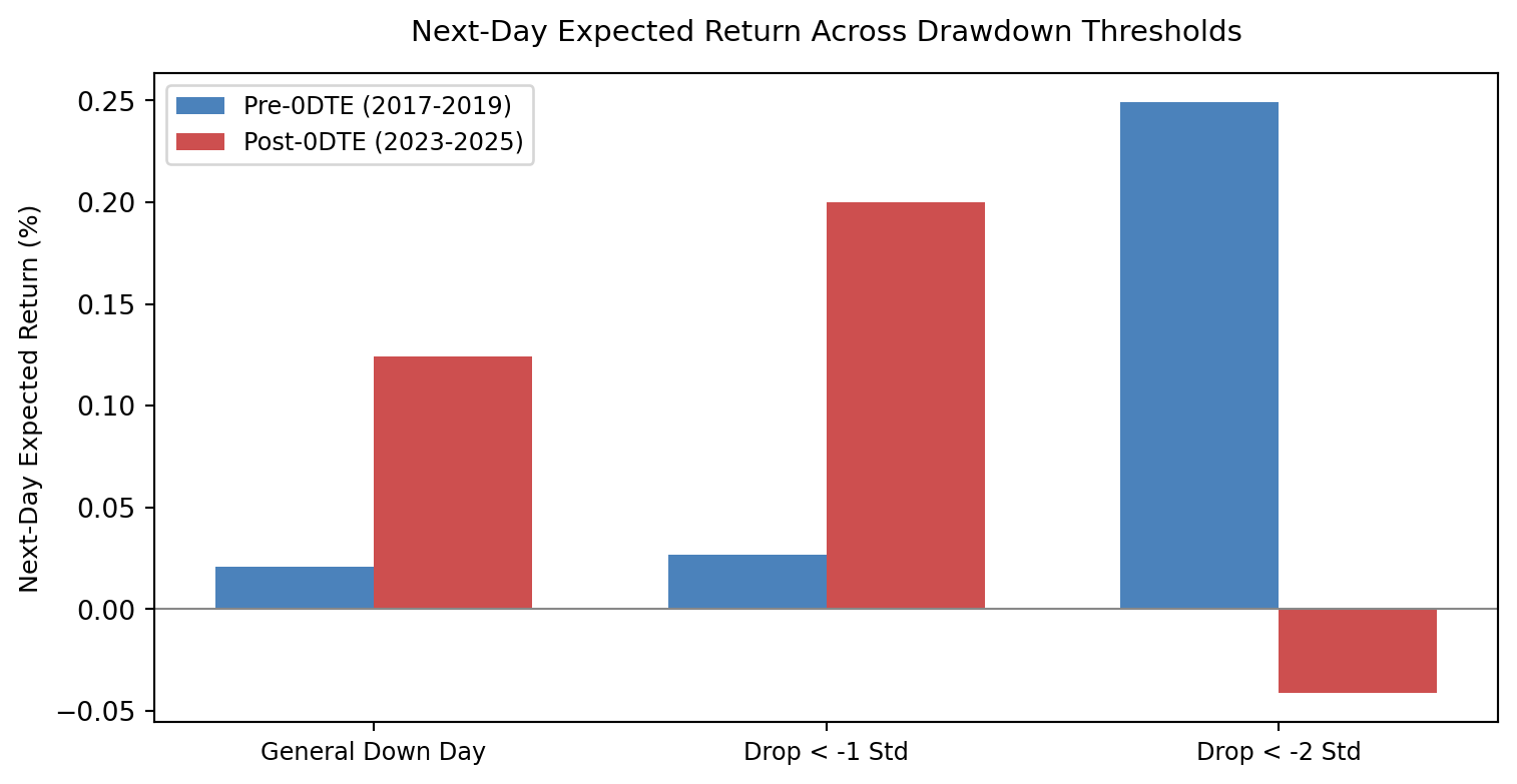

Result Interpretation:

• Conditional rebound probability \(P(R_t > 0 \mid R_{t-1} < 0)\) shows modest variation across regimes: 57.01% in Pre-0DTE vs. 57.93% in Post-0DTE (+0.92%p difference). The directional frequency of positive days following a drop remains near historical base rates.
• Expected return magnitude following drawdowns expands sharply. Following an unconditioned down day, next-day expected return increases from +0.021% to +0.124% (a sixfold gain).
• After a one-standard-deviation selloff (\(R_{t-1} < -\sigma\)), next-day expected return surges from +0.027% (Pre) to +0.200% (Post), an expansion of over sevenfold. Dip-buying flows and dealer delta hedging trigger stronger immediate positive price adjustments rather than cascade selling.

Hypothesis 2 Evaluation:

• Hypothesis 2 posited that conditional rebound probability and mean bounce magnitude following drawdowns would expand in the post-0DTE regime.
• Binary directional probability \(P(R_t > 0 \mid R_{t-1} < 0)\) displayed negligible shift (+0.92%p). In contrast, rebound elasticity measured by expected drift magnitude (\(E[R_t \mid R_{t-1} < -\sigma]\)) increased sevenfold (+0.200% vs. +0.027%). Hypothesis 2 is supported primarily through return magnitude rather than binary transition frequency.

5.4 Interaction Regression Estimation

An interaction regression assesses whether higher 0DTE market share (\(W_t\)) directly amplifies the rebound magnitude conditional on prior-day losses.

comb = pd.concat([pre_df, post_df])
comb['W_t'] = np.where(comb.index >= '2023-01-01', 0.48, 0.08)
comb['is_down'] = (comb['ret_lag'] < 0).astype(int)
comb['down_ret'] = comb['ret_lag'] * comb['is_down']
comb['interact'] = comb['down_ret'] * comb['W_t']

ols_res = smf.ols('ret ~ ret_lag + down_ret + interact', data=comb).fit(
    cov_type='HAC', cov_kwds={'maxlags': 5}
)

pd.DataFrame({
    'Coefficient': ols_res.params,
    'Std Error (HAC)': ols_res.bse,
    't-statistic': ols_res.tvalues,
    'p-value': ols_res.pvalues
}).round(4)

	Coefficient	Std Error (HAC)	t-statistic	p-value
Intercept	0.0007	0.0004	1.5234	0.1277
ret_lag	-0.0380	0.0873	-0.4350	0.6636
down_ret	-0.0226	0.1459	-0.1551	0.8767
interact	0.0868	0.3169	0.2739	0.7842

Result Interpretation and Microstructure Limitations:

• Prior-day return coefficient (\(\beta_1 = -0.0380\)) captures baseline mean reversion, though not statistically significant at conventional levels (\(p = 0.664\)).
• Downside dummy interaction coefficient (\(\beta_3 = 0.0868\), \(p = 0.784\)) does not achieve statistical significance under daily close-to-close returns.
• Close-to-close daily resolution averages out intraday dealer rebalancing flows, which peak during the final two hours of trading (14:00-16:00 ET). Unconditioned higher moments clearly capture the regime shift, but identifying causal elasticity solely via low-frequency daily closes without intraday dealer net gamma inventory remains statistically limited.

5.5 Hypothesis Evaluation Summary

Hypothesis	Evaluated Metric	Pre-0DTE	Post-0DTE	Empirical Finding	Verdict
H1: Rightward Skewness	Skewness (\(S\))	-0.701	+0.329	+1.030 shift toward positive skew; KS test rejects equality (\(p=0.0078\))	Supported
H2a: Directional Probability	\(P(R_t > 0 \mid R_{t-1} < 0)\)	57.01%	57.93%	+0.92%p difference (within standard confidence bands)	Inconclusive
H2b: Rebound Magnitude	\(E[R_t \mid R_{t-1} < -\sigma]\)	+0.027%	+0.200%	Rebound drift expanded 7.4-fold following moderate drops	Supported
H2c: OLS Interaction	Interaction \(\beta_3\)	N/A	\(\beta_3 = 0.0868\)	Statistically insignificant at daily close-to-close resolution (\(p=0.784\))	Data-constrained

6 Limitations and Confounding Factors

• Generative AI capex cycle: mega-cap tech earnings power (M7) drove fundamental dip-buying flows from 2023 onward, potentially confounding purely microstructure-driven upside drift.
• Passive 401(k) inflows and corporate buybacks: automated retirement inflows and ongoing corporate share repurchases provide an underlying structural floor to spot indices.
• Daily aggregation limits: 0DTE delta rebalancing peaks in the final two hours of trading (14:00-16:00 ET). Close-to-close metrics net out intraday reversals and may understate microstructure impact.
• Lack of dealer net gamma direction: 0DTE trading includes institutional short-volatility strategies (e.g., iron condors) alongside directional call buying. Gross volume share cannot distinguish net long gamma from net short gamma.

7 Conclusion

Empirical examination identifies structural shifts in S&P 500 daily returns following the full rollout of 0DTE index options in 2022:

• Distributional transformation: daily return skewness shifted from negative (-0.701) to positive (+0.329), while excess kurtosis increased from 5.418 to 14.165. The two-sample Kolmogorov-Smirnov test confirmed structural non-equivalence at the 1% significance level (\(p = 0.0078\)).
• Rebound elasticity expansion: directional transition probabilities (\(P(R_t > 0 \mid R_{t-1} < 0)\)) showed marginal change (57.01% to 57.93%), but expected return magnitude following moderate drops (\(R_{t-1} < -\sigma\)) surged from +0.027% to +0.200%. Systematic downside cascade selling was replaced by rapid V-shaped dip-buying recoveries.
• Identification boundaries: daily close-to-close metrics cannot isolate intraday dealer gamma rebalancing occurring near the market close, indicating that future research requires high-frequency tick data and signed order flows.

Institutionalization of five-day daily expirations has altered spot price dynamics, converting traditional left-tail decay into compressed, right-leaning volatility with amplified downside shock absorption.