Appendix: Weighting

Author

gitSAM

Published

September 15, 2026

1 Discrete Rank-based Convex Weighting Scheme

In the TBTF framework, asset allocation within the top-decile state (\(\text{State} = 10\)) departs from classical linear risk-beta pricing. Instead, capital weights \(w_i\) are determined through structural specifications capturing the convex relationship between market capitalization rank \(r_i\) and capital share:

\[ w_i \propto f(r_i; \boldsymbol{\theta}) \]

where \(r_i \in \{1, 2, \dots, n\}\) denotes the intra-state rank (\(r=1\) being the smallest within the top-\(n\), and \(r=n\) being the largest mega-cap firm), and \(\sum_{i=1}^n w_i = 1\).

We investigate three representative weighting paradigms:

  • Parametric: Exponential Form (\(w_i \propto \alpha e^{\beta r_i}\))
  • Nonparametric: Median-Based (\(\hat{w}_r \propto \text{Median}(w_{r,t})\))
  • Semi-Parametric: Zipf Fit (\(w(k_i; \alpha) \propto k_i^{-\alpha}\) calibrated to top-\(m\) concentration \(C_m\), evaluated for \(m=1\) and \(m=3\))

Exclusion of Quadratic Form: While polynomial formulations such as \(w_i \propto \alpha + \beta r_i + \gamma r_i^2\) are commonly considered in unconstrained curve fitting, the quadratic specification can easily violate monotonicity (\(\frac{\partial w}{\partial r} < 0\) at lower ranks) and may assign counter-intuitively higher weights to firms with the smallest capital shares. In portfolio execution, such non-monotonic turning points induce excessive turnover and trading friction. Therefore, the quadratic form is deliberately excluded from this comparative framework in favor of structurally monotonic designs.

Code
import sys
import os
import sqlite3
import numpy as np
import pandas as pd
import matplotlib.pyplot as plt
import statsmodels.api as sm
from scipy.optimize import root_scalar

sys.path.append(os.path.abspath('../data/'))
import tbtf

# Load CRSP dataset
con = sqlite3.connect(database="../data/tbtf.sqlite")
crsp = pd.read_sql_query(
    sql="SELECT * FROM crsp",
    con=con,
    parse_dates={"date"}
)
con.close()

2 Specifications

2.1 Parametric: Exponential Form

\[ w_i \propto \alpha e^{\beta r_i} \quad \Longleftrightarrow \quad \ln(w_i) = \ln(\alpha) + \beta r_i \]

  • Estimation: Log-linear OLS regression of \(\ln(\text{capshare}_i)\) on intra-state rank \(r_i\).
  • Curvature: The coefficient \(\beta > 0\) governs the exponential growth rate across ranks.
  • Structural Properties: Guarantees strict positivity (\(w_i > 0, \forall i\)) and strict monotonicity (\(\frac{\partial w}{\partial r} > 0\)). It aligns naturally with scale-invariant compounding processes and power-law distribution tails.

2.2 Nonparametric: Median-Based Estimation

\[ \hat{w}_r \propto \text{Median}\left(\{w_{r,t}\}_{t=1}^T\right), \quad \sum_{r=1}^n \hat{w}_r = 1 \]

  • Estimates the rank-specific central tendency directly from historical in-sample medians without imposing functional or structural curvature assumptions.
  • By using medians rather than sample means, this estimator remains robust against transient market cap spikes and monthly distributional outliers.

2.3 Semi-Parametric: Zipf Fit

The Generalized Zipf Fit extends the fixed exponent (\(\zeta = 1\)) of the base Zipf model (standard Harmonic Number Weighting) to an adjustable parameter \(\alpha \ge 0\). The single parameter \(\alpha\) is calibrated so that the cumulative model weight of the top-\(m\) assets exactly matches the observed in-sample capital share concentration \(C_m\).

Mathematical Formulation & Estimation Details (Click to expand)

2.3.1 Mathematical Formulation

Let descending rank be denoted by \(k_i = n - r_i + 1\) (where \(k_1 = 1\) is the largest mega-cap firm and \(k_n = n\) is the smallest in the top-\(n\)). The weight allocated to rank \(k_i\) is given by:

\[ w(k_i; \alpha) = \frac{k_i^{-\alpha}}{\sum_{j=1}^n j^{-\alpha}} = \frac{k_i^{-\alpha}}{H_{n, \alpha}} \]

where \(H_{n, \alpha} = \sum_{j=1}^n j^{-\alpha}\) is the generalized harmonic number of order \(\alpha\).

2.3.2 Calibration Mechanism

Given the observed in-sample capital share vector \(s = (s_1, s_2, \dots, s_n)\) sorted in descending order of market capitalization, the top-\(m\) concentration ratio is defined as:

\[ C_m = \sum_{j=1}^m s_j \]

The parameter \(\hat{\alpha}\) is determined by matching the cumulative weight of the top-\(m\) assets to \(C_m\):

\[ f(\alpha) = \frac{H_{m, \alpha}}{H_{n, \alpha}} = \frac{\sum_{j=1}^m j^{-\alpha}}{\sum_{j=1}^n j^{-\alpha}} = C_m \]

When \(m = 1\) (single apex anchor), \(H_{1, \alpha} = 1^{-\alpha} = 1\) identically for all \(\alpha\). Consequently, the calibration condition simplifies to:

\[ f(\alpha) = \frac{1}{H_{n, \alpha}} = s_1 \quad \Longleftrightarrow \quad H_{n, \alpha} = \frac{1}{s_1} \]

In other words, when \(m = 1\), the estimation of \(\alpha\) reduces to finding the root where the generalized harmonic number \(H_{n, \alpha}\) equals the exact reciprocal of the top asset’s empirical capital share (\(1/s_1\)), providing a transparent and intuitive link between the apex share and the global decay exponent.

2.3.3 Monotonicity and Uniqueness of Solution

For \(\alpha \in [0, \infty)\), the concentration ratio function \(f(\alpha)\) exhibits the following properties:

  • Equal Weighting boundary: As \(\alpha \to 0\), \(f(0) = \frac{m}{n}\).
  • Monopoly boundary: As \(\alpha \to \infty\), \(f(\infty) = 1\) (100% allocation to the top asset \(k=1\)).
  • Strict Monotonicity: \(\frac{d}{d\alpha} f(\alpha) > 0\) holds strictly for all \(\alpha \ge 0\) when \(1 \le m < n\).

Under realistic market conditions where the empirical top-\(m\) share satisfies \(\frac{m}{n} < C_m < 1\), the Intermediate Value Theorem and strict monotonicity guarantee a unique root \(\hat{\alpha}\).

2.3.4 Numerical Solution Procedure

Because \(f(\alpha) - C_m = 0\) does not possess a closed-form analytic solution, 1D root-finding (Brent’s method) is applied:

  1. Target Calculation: Compute \(C_m = \sum_{j=1}^m s_j\) from in-sample median shares.
  2. Bracketing: Search within \([\alpha_{\min}, \alpha_{\max}] = [0.001, 5.0]\), which covers all empirical equity market conditions.
  3. Root Finding: Brent’s method converges to machine precision within a few iterations.

2.3.5 Structural Interpretation of Parameter Magnitude

  • \(\hat{\alpha} < 1\): Observed concentration is milder than the base Zipf model (\(\alpha = 1\)). The model dampens apex curvature, avoiding over-allocation to the top rank.
  • \(\hat{\alpha} = 1\): Empirical concentration exactly coincides with the base Zipf model (\(\frac{H_{m, 1}}{H_{n, 1}} = \frac{H_m}{H_n}\)).
  • \(\hat{\alpha} > 1\): Apex concentration exceeds the base harmonic decay, reflecting extreme power-law dominance.
Code
in_sample_months = 48

df_2009, _ = tbtf.split_in_out_sample(crsp, '2009-12-31', in_sample_months)
df_2023, _ = tbtf.split_in_out_sample(crsp, '2023-12-31', in_sample_months)

def plot_median_fit(df_in_sample, n=10, state=10, ax=None):
    all_obs = []
    for date, group in df_in_sample[df_in_sample['state'] == state].groupby('date'):
        g = group.sort_values('mktcap_lag', ascending=False).head(n).copy()
        if len(g) < n: continue
        g = g.sort_values('mktcap_lag')
        g['rank'] = np.arange(1, n + 1)
        g['capshare'] = g['mktcap_lag'] / g['mktcap_lag'].sum()
        all_obs.append(g[['rank', 'capshare']])
    df_all = pd.concat(all_obs, ignore_index=True)
    df_median = df_all.groupby('rank')['capshare'].median().reset_index()
    
    if ax is None:
        fig, ax = plt.subplots(figsize=(8, 5))
    ax.scatter(df_all['rank'], df_all['capshare'], alpha=0.4, label='Observed', color='gray')
    ax.step(df_median['rank'], df_median['capshare'], where='mid', linewidth=2.5, color='blue', label='Median Capshare')
    ax.set_xlabel("Rank (1 = Smallest, 10 = Largest)")
    ax.set_ylabel("Capital Share")
    ax.set_xticks(np.arange(1, n + 1))
    ax.legend()
    ax.grid(True)
    return ax

def fit_and_plot_zipf(df_in_sample, n=10, m=3, state=10, ax=None, color='teal'):
    all_obs = []
    for date, group in df_in_sample[df_in_sample['state'] == state].groupby('date'):
        g = group.sort_values('mktcap_lag', ascending=False).head(n).copy()
        if len(g) < n: continue
        g = g.sort_values('mktcap_lag')
        g['rank'] = np.arange(1, n + 1)
        g['capshare'] = g['mktcap_lag'] / g['mktcap_lag'].sum()
        all_obs.append(g[['rank', 'capshare']])
    df_all = pd.concat(all_obs, ignore_index=True)
    
    median_shares = df_all.groupby('rank')['capshare'].median()
    s = (median_shares / median_shares.sum()).sort_index(ascending=False).values
    C_m = s[:m].sum()
    
    def obj(alpha):
        h_m = np.sum(np.arange(1, m + 1) ** (-alpha))
        h_n = np.sum(np.arange(1, n + 1) ** (-alpha))
        return (h_m / h_n) - C_m
    
    res = root_scalar(obj, bracket=[0.001, 5.0], method='brentq')
    alpha_hat = res.root
    
    ranks = np.arange(1, n + 1)
    k = n - ranks + 1
    w_zipf = (k ** (-alpha_hat)) / np.sum(k ** (-alpha_hat))
    
    if ax is None:
        fig, ax = plt.subplots(figsize=(8, 5))
    ax.scatter(df_all['rank'], df_all['capshare'], alpha=0.4, label='Observed', color='gray')
    ax.step(ranks, w_zipf, where='mid', linewidth=2.5, color=color, label=f'Zipf Fit ($\\hat{{\\alpha}}={alpha_hat:.3f}, C_{m}={C_m:.3f}$)')
    ax.scatter(ranks, w_zipf, color=color, s=35, zorder=3)
    ax.set_xlabel("Rank (1 = Smallest, 10 = Largest)")
    ax.set_ylabel("Capital Weight")
    ax.set_xticks(ranks)
    ax.grid(True, linestyle='--', alpha=0.6)
    ax.legend()
    return ax, alpha_hat, C_m

fig, axes = plt.subplots(4, 2, figsize=(14, 20))

# 1. Parametric: Exponential Fit
tbtf.plot_exponential_fit(df_2009, n=10, state=10, ax=axes[0, 0])
axes[0, 0].set_title("Pre-2010: Exponential Fit (Snapshot 2009-12-31)")

tbtf.plot_exponential_fit(df_2023, n=10, state=10, ax=axes[0, 1])
axes[0, 1].set_title("Post-2010: Exponential Fit (Snapshot 2023-12-31)")

# 2. Nonparametric: Median-Based Fit
plot_median_fit(df_2009, n=10, state=10, ax=axes[1, 0])
axes[1, 0].set_title("Pre-2010: Median-Based Capshare (Snapshot 2009-12-31)")

plot_median_fit(df_2023, n=10, state=10, ax=axes[1, 1])
axes[1, 1].set_title("Post-2010: Median-Based Capshare (Snapshot 2023-12-31)")

# 3. Semi-Parametric: Zipf Fit (m = 1)
_, a_pre_m1, _ = fit_and_plot_zipf(df_2009, n=10, m=1, state=10, ax=axes[2, 0], color='seagreen')
axes[2, 0].set_title(f"Pre-2010: Zipf Fit with $m=1$ ($\\hat{{\\alpha}}={a_pre_m1:.3f}$)")

_, a_post_m1, _ = fit_and_plot_zipf(df_2023, n=10, m=1, state=10, ax=axes[2, 1], color='seagreen')
axes[2, 1].set_title(f"Post-2010: Zipf Fit with $m=1$ ($\\hat{{\\alpha}}={a_post_m1:.3f}$)")

# 4. Semi-Parametric: Zipf Fit (m = 3)
_, a_pre_m3, _ = fit_and_plot_zipf(df_2009, n=10, m=3, state=10, ax=axes[3, 0], color='darkcyan')
axes[3, 0].set_title(f"Pre-2010: Zipf Fit with $m=3$ ($\\hat{{\\alpha}}={a_pre_m3:.3f}$)")

_, a_post_m3, _ = fit_and_plot_zipf(df_2023, n=10, m=3, state=10, ax=axes[3, 1], color='darkcyan')
axes[3, 1].set_title(f"Post-2010: Zipf Fit with $m=3$ ($\\hat{{\\alpha}}={a_post_m3:.3f}$)")

plt.tight_layout()
plt.show()
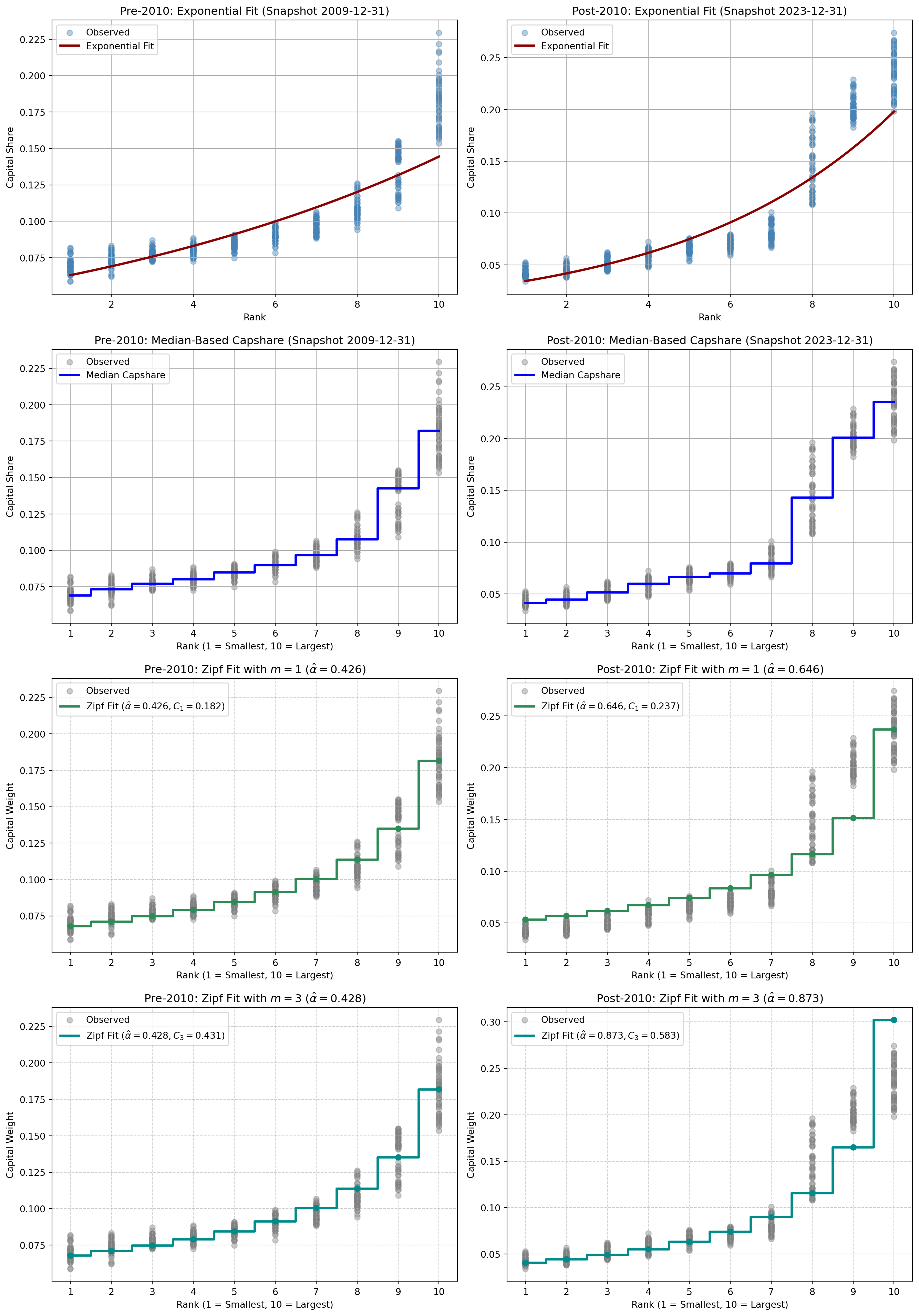
Pre-2010 vs. Post-2010 Fits across Weighting Schemes

3 Comparison

Code
def compute_weighting_schemes(df_in_sample, n=10, state=10):
    all_obs = []
    for date, group in df_in_sample[df_in_sample['state'] == state].groupby('date'):
        g = group.sort_values('mktcap_lag', ascending=False).head(n).copy()
        if len(g) < n: continue
        g = g.sort_values('mktcap_lag')
        g['rank'] = np.arange(1, n + 1)
        g['capshare'] = g['mktcap_lag'] / g['mktcap_lag'].sum()
        all_obs.append(g[['rank', 'capshare']])
    
    df_all = pd.concat(all_obs, ignore_index=True)
    ranks = np.arange(1, n + 1)
    k = n - ranks + 1
    
    # 1. Exponential fit
    df_all['log_capshare'] = np.log(df_all['capshare'])
    X_exp = sm.add_constant(df_all['rank'])
    model_exp = sm.OLS(df_all['log_capshare'], X_exp).fit()
    w_exp = np.exp(model_exp.params['const'] + model_exp.params['rank'] * ranks)
    w_exp = w_exp / w_exp.sum()
    
    # 2. Median-Based fit
    w_med_raw = df_all.groupby('rank')['capshare'].median().values
    w_median = w_med_raw / w_med_raw.sum()
    
    # 3. Mean-Based fit
    w_mean_raw = df_all.groupby('rank')['capshare'].mean().values
    w_mean = w_mean_raw / w_mean_raw.sum()
    
    # Helper to calibrate Zipf Fit
    s = w_median[::-1]
    def solve_zipf(m_val):
        C_m = s[:m_val].sum()
        def obj(alpha):
            h_m = np.sum(np.arange(1, m_val + 1) ** (-alpha))
            h_n = np.sum(np.arange(1, n + 1) ** (-alpha))
            return (h_m / h_n) - C_m
        res = root_scalar(obj, bracket=[0.001, 5.0], method='brentq')
        alpha_hat = res.root
        weights = (k ** (-alpha_hat)) / np.sum(k ** (-alpha_hat))
        return weights, alpha_hat, C_m
    
    w_zipf_m1, alpha_m1, c_m1 = solve_zipf(1)
    w_zipf_m3, alpha_m3, c_m3 = solve_zipf(3)
    
    weights_df = pd.DataFrame({
        'Rank': ranks,
        'Exponential': w_exp,
        'Median-Based': w_median,
        'Mean-Based': w_mean,
        'Zipf Fit (m=1)': w_zipf_m1,
        'Zipf Fit (m=3)': w_zipf_m3
    }).set_index('Rank')
    
    calib_info = {
        'alpha_m1': alpha_m1, 'c_m1': c_m1,
        'alpha_m3': alpha_m3, 'c_m3': c_m3
    }
    return weights_df, df_all, calib_info

weights_pre, obs_pre, info_pre = compute_weighting_schemes(df_2009, n=10, state=10)
weights_post, obs_post, info_post = compute_weighting_schemes(df_2023, n=10, state=10)

3.1 Allocation Comparison Table

Code
df_table = pd.concat({
    'Pre-2010': weights_pre[['Exponential', 'Median-Based', 'Zipf Fit (m=1)', 'Zipf Fit (m=3)']],
    'Post-2010': weights_post[['Exponential', 'Median-Based', 'Zipf Fit (m=1)', 'Zipf Fit (m=3)']]
}, axis=1)
df_table.round(4)
Pre-2010 Post-2010
Exponential Median-Based Zipf Fit (m=1) Zipf Fit (m=3) Exponential Median-Based Zipf Fit (m=1) Zipf Fit (m=3)
Rank
1 0.0638 0.0688 0.0680 0.0679 0.0358 0.0416 0.0535 0.0405
2 0.0700 0.0730 0.0712 0.0710 0.0435 0.0452 0.0573 0.0444
3 0.0767 0.0768 0.0748 0.0747 0.0528 0.0519 0.0618 0.0492
4 0.0841 0.0798 0.0792 0.0791 0.0642 0.0604 0.0674 0.0553
5 0.0922 0.0846 0.0846 0.0845 0.0780 0.0672 0.0745 0.0633
6 0.1011 0.0896 0.0914 0.0914 0.0947 0.0705 0.0838 0.0742
7 0.1109 0.0964 0.1005 0.1005 0.1151 0.0801 0.0968 0.0901
8 0.1216 0.1073 0.1136 0.1137 0.1398 0.1440 0.1165 0.1158
9 0.1333 0.1420 0.1351 0.1352 0.1698 0.2022 0.1514 0.1650
10 0.1462 0.1815 0.1815 0.1819 0.2063 0.2369 0.2369 0.3022

3.2 Regime Comparison Plots: All Schemes

Code
fig, axes = plt.subplots(1, 2, figsize=(16, 6))

colors = {
    'Exponential': 'darkred',
    'Median-Based': 'royalblue',
    'Zipf Fit (m=1)': 'seagreen',
    'Zipf Fit (m=3)': 'darkcyan'
}
markers = {
    'Exponential': 'o',
    'Median-Based': '^',
    'Zipf Fit (m=1)': 's',
    'Zipf Fit (m=3)': 'D'
}

# Pre-2010
axes[0].scatter(obs_pre['rank'], obs_pre['capshare'], color='gray', alpha=0.25, 
                s=25, label='Observed Capshare', zorder=1)
for col in ['Exponential', 'Median-Based', 'Zipf Fit (m=1)', 'Zipf Fit (m=3)']:
    axes[0].plot(weights_pre.index, weights_pre[col], marker=markers[col], 
                 color=colors[col], label=col, linewidth=2, zorder=3)
axes[0].set_title(
    f"Pre-2010 Regime (Snapshot 2009-12-31)\n$\\hat{{\\alpha}}_{{m=1}}={info_pre['alpha_m1']:.3f},\\ \\hat{{\\alpha}}_{{m=3}}={info_pre['alpha_m3']:.3f}$", 
    fontsize=12
)
axes[0].set_xlabel("Rank (1 = Smallest in Top-10, 10 = Largest Mega-Cap)")
axes[0].set_ylabel("Portfolio Weight / Capital Share")
axes[0].set_xticks(np.arange(1, 11))
axes[0].grid(True, linestyle='--', alpha=0.6)
axes[0].legend()

# Post-2010
axes[1].scatter(obs_post['rank'], obs_post['capshare'], color='gray', alpha=0.25, 
                s=25, label='Observed Capshare', zorder=1)
for col in ['Exponential', 'Median-Based', 'Zipf Fit (m=1)', 'Zipf Fit (m=3)']:
    axes[1].plot(weights_post.index, weights_post[col], marker=markers[col], 
                 color=colors[col], label=col, linewidth=2, zorder=3)
axes[1].set_title(
    f"Post-2010 Regime (Snapshot 2023-12-31)\n$\\hat{{\\alpha}}_{{m=1}}={info_post['alpha_m1']:.3f},\\ \\hat{{\\alpha}}_{{m=3}}={info_post['alpha_m3']:.3f}$", 
    fontsize=12
)
axes[1].set_xlabel("Rank (1 = Smallest in Top-10, 10 = Largest Mega-Cap)")
axes[1].set_ylabel("Portfolio Weight / Capital Share")
axes[1].set_xticks(np.arange(1, 11))
axes[1].grid(True, linestyle='--', alpha=0.6)
axes[1].legend()

plt.tight_layout()
plt.show()

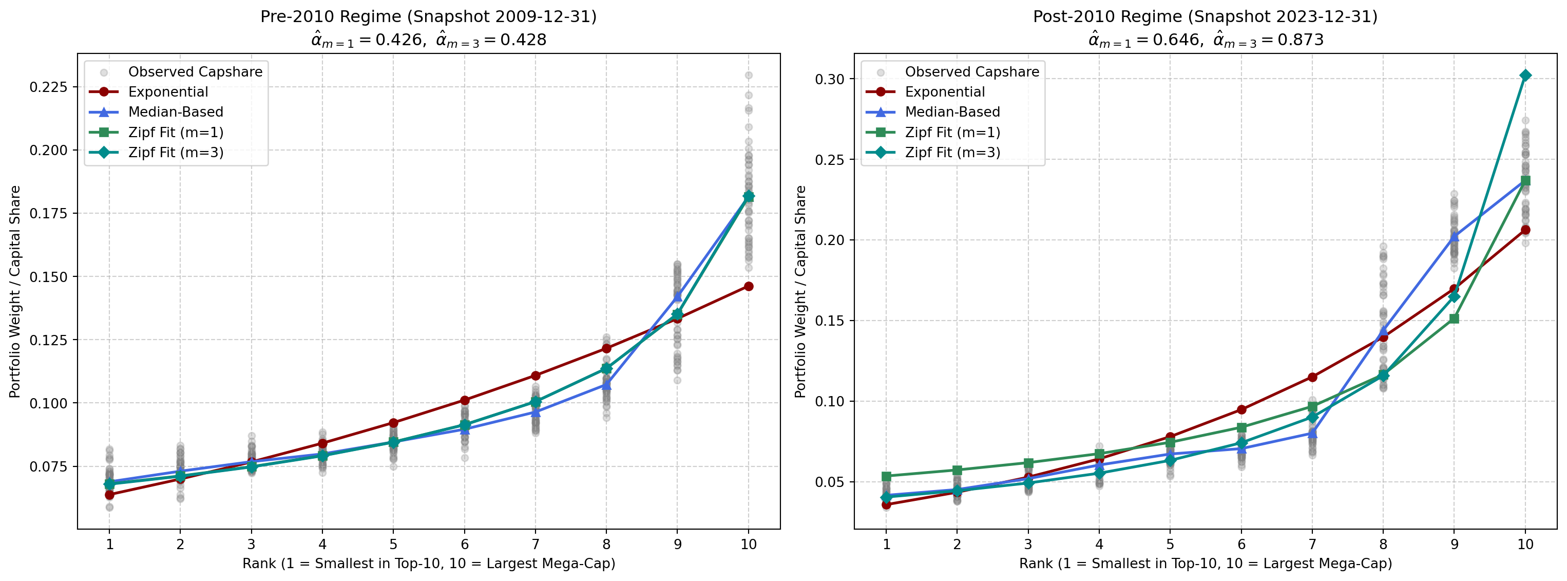
Comparison of Weighting Schemes with Observed Capital Shares across Pre-2010 and Post-2010 Regimes

3.3 Structural Findings

  1. Regime Shift Captured by Zipf Parameter \(\hat{\alpha}\):
    • Pre-2010 Regime: Calibrated parameters are \(\hat{\alpha}_{m=1} \approx 0.426\) and \(\hat{\alpha}_{m=3} \approx 0.428\). Both values are substantially below 1, indicating that capital concentration in the pre-2010 era was far less convex than implied by the base Zipf model (\(\alpha = 1\)). The consistency between \(m=1\) and \(m=3\) suggests a uniform power-law tail across the top ranks.
    • Post-2010 Regime: Calibrated exponents increase markedly to \(\hat{\alpha}_{m=1} \approx 0.646\) and \(\hat{\alpha}_{m=3} \approx 0.873\). This twofold rise reflects the rapid institutional concentration of capital into mega-cap incumbents, driving the real market distribution significantly closer to the base Zipf model.
    • The wedge between \(\hat{\alpha}_{m=3}\) (\(0.873\)) and \(\hat{\alpha}_{m=1}\) (\(0.646\)) post-2010 demonstrates that capital accumulation is concentrated across the collective top-3 cluster (e.g., AAPL, MSFT, NVDA) rather than resting exclusively in a single firm.
  2. Structural Robustness Across Paradigms:
    • Exponential Form (Parametric) provides smooth convexity and global monotonicity across all ranks, effectively interpolating mid-tier ranks (\(r = 4 \sim 8\)).
    • Median-Based (Nonparametric) serves as a model-free benchmark reflecting the realized median capital structure, immune to distributional assumptions.
    • Zipf Fit (Semi-Parametric) combines the parsimony of power-law physics with empirical adaptability, controlling the entire portfolio allocation curve through a single observable concentration metric (\(C_1\) or \(C_3\)).

3.4 Practical Implications

From an implementation and trading perspective, the theoretical properties of these weighting schemes yield distinct performance and execution trade-offs:

  1. The Opportunity Cost of Parametric Smoothing (Exponential Form): The exponential form enforces log-linear regularity (\(\ln w_i \propto \beta r_i\)), which acts as a rigid structural constraint. In the post-2010 data, the Exponential model allocates \(35.2\%\) of the portfolio to mid-tier firms (ranks 4–7) while granting only \(37.6\%\) to the top-2 mega-caps (ranks 9–10). In contrast, the empirical median market distribution allocates \(43.9\%\) to the top-2 and only \(27.8\%\) to the mid-tier. By over-allocating capital to the “middle class” of the top-decile firms, the exponential weighting fails to fully capture the structural wealth polarization occurring at the extreme tail. In a regime driven by capital lock-in at the very apex, this induces substantial opportunity costs relative to the true capital flow dynamics.

  2. The Turnover Fragility of Apex Calibration (Zipf Fit): While the Zipf Fit effectively reveals the intensification of structural capital pooling—demonstrated by the sharp bifurcation between \(m=1\) (\(\hat{\alpha} = 0.646\)) and \(m=3\) (\(\hat{\alpha} = 0.873\)) post-2010—it relies on matching extreme boundary shares (\(s_1\) or \(s_1 + s_2 + s_3\)). In live trading, calibrating a global exponent to extreme boundary statistics can cause high parameter volatility. Monthly fluctuations in the market cap of the top 1–3 firms propagate across all \(n\) portfolio weights, generating elevated portfolio turnover and transaction costs.

  3. Optimality of Nonparametric Weighting in Practice: The Median-Based nonparametric scheme directly accommodates structural wealth polarization without rigid parametric distortion: it assigns \(43.9\%\) to ranks 9–10, closely mirroring the empirical market concentration. Furthermore, because the sample median ignores extreme monthly spikes and avoids re-estimating sensitive global curvature parameters, it offers an insensitive, robust allocation profile. Consequently, for practical execution, the nonparametric median-based scheme presents the nice balance: it rides the tailwind of structural capital concentration while minimizing estimation risk and turnover friction.

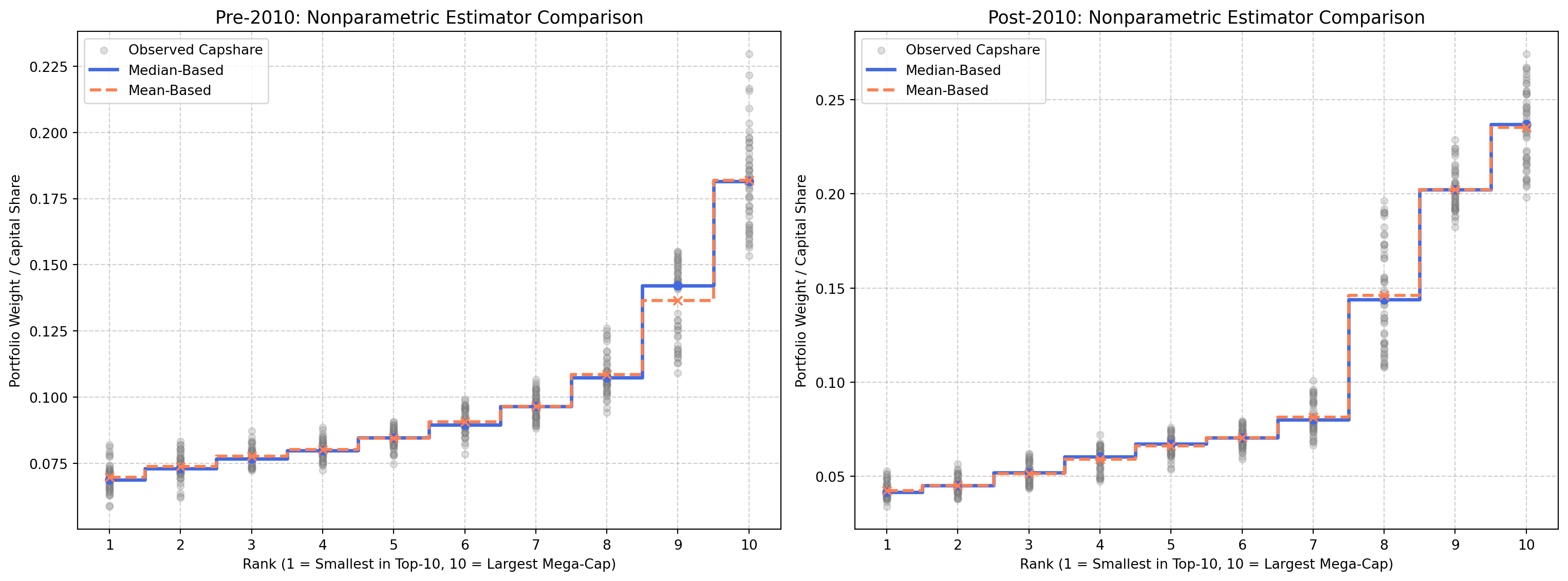
3.5 Comparison of Nonparametric Estimators: Median vs. Mean

To examine how the central tendency is constructed in the nonparametric framework, we directly compare the Median-Based and Mean-Based capital share curves against the observed data across both regimes.

Code
fig, axes = plt.subplots(1, 2, figsize=(16, 6))

# Pre-2010
axes[0].scatter(obs_pre['rank'], obs_pre['capshare'], color='gray', alpha=0.25, 
                s=25, label='Observed Capshare', zorder=1)
axes[0].step(weights_pre.index, weights_pre['Median-Based'], where='mid', 
             color='royalblue', linewidth=2.5, label='Median-Based', zorder=3)
axes[0].scatter(weights_pre.index, weights_pre['Median-Based'], color='royalblue', s=35, zorder=3)
axes[0].step(weights_pre.index, weights_pre['Mean-Based'], where='mid', 
             color='coral', linestyle='--', linewidth=2.2, label='Mean-Based', zorder=3)
axes[0].scatter(weights_pre.index, weights_pre['Mean-Based'], color='coral', marker='x', s=40, zorder=3)

axes[0].set_title("Pre-2010: Nonparametric Estimator Comparison", fontsize=13)
axes[0].set_xlabel("Rank (1 = Smallest in Top-10, 10 = Largest Mega-Cap)")
axes[0].set_ylabel("Portfolio Weight / Capital Share")
axes[0].set_xticks(np.arange(1, 11))
axes[0].grid(True, linestyle='--', alpha=0.6)
axes[0].legend()

# Post-2010
axes[1].scatter(obs_post['rank'], obs_post['capshare'], color='gray', alpha=0.25, 
                s=25, label='Observed Capshare', zorder=1)
axes[1].step(weights_post.index, weights_post['Median-Based'], where='mid', 
             color='royalblue', linewidth=2.5, label='Median-Based', zorder=3)
axes[1].scatter(weights_post.index, weights_post['Median-Based'], color='royalblue', s=35, zorder=3)
axes[1].step(weights_post.index, weights_post['Mean-Based'], where='mid', 
             color='coral', linestyle='--', linewidth=2.2, label='Mean-Based', zorder=3)
axes[1].scatter(weights_post.index, weights_post['Mean-Based'], color='coral', marker='x', s=40, zorder=3)

axes[1].set_title("Post-2010: Nonparametric Estimator Comparison", fontsize=13)
axes[1].set_xlabel("Rank (1 = Smallest in Top-10, 10 = Largest Mega-Cap)")
axes[1].set_ylabel("Portfolio Weight / Capital Share")
axes[1].set_xticks(np.arange(1, 11))
axes[1].grid(True, linestyle='--', alpha=0.6)
axes[1].legend()

plt.tight_layout()
plt.show()

Comparison of Nonparametric Estimators: Median-Based vs. Mean-Based