Corner Solutions

Convex in Optimization Model, but Non-Convex in Reality

Abstract

This notebook explores the corner solution problem in optimization theory, where theoretical convexity contrasts with real-world non-convexities. Through insightful examples, it demonstrates how economic and mathematical assumptions can diverge in practice.

Keywords

corner solution, optimization, convex, non-convex

1 Introduction

In standard economic theory, both consumer preferences and production sets are generally assumed to exhibit convexity (Arrow and Debreu 1954; Debreu 1959). This assumption supports foundational results, including the existence and uniqueness of equilibrium and the efficiency of market allocations. In practice, however, features such as network externalities (Katz and Shapiro 1985; Rochet and Tirole 2003), rent-seeking (Shleifer and Vishny 1993), and multiple equilibria—often culminating in pronounced market dominance—can produce outcomes resembling non-convex preferences (Arthur 1994). In many cases, corner solutions and path-dependent equilibria emerge from winner-takes-all dynamics, concentrated economic power, and barriers to entry.

2 Convexity in Economic Theory

2.1 Convex Preferences and Production Sets

• Consumer preferences are typically modeled with quasi-concave utility functions, yielding convex (or “bowl-shaped”) indifference curves. This setup implies a preference for diversity in consumption, rather than extreme or corner solutions (Debreu 1959).
• Producers are often assumed to face diminishing marginal returns, reflected in a convex production possibility set. Under such conditions, output expansions follow a predictable pattern, and average costs rise eventually.

2.2 Existence and Efficiency of Equilibrium

• With convexity, free market entry, symmetric information, and price-taking behavior, perfectly competitive markets are shown to possess a stable equilibrium that is Pareto efficient (Arrow and Debreu 1954).
• These results typically rely on fixed-point theorems and the properties of convex sets, ensuring both the existence of equilibrium prices and (in many cases) uniqueness or stability (Debreu 1959).

2.3 Normative Implications

• Convexity underpins the normative stance that, absent significant market failures, competitive markets gravitate toward Pareto-efficient resource allocations.
• Consequently, government interventions usually aim to correct externalities, public goods issues, or information asymmetries within a broader context of largely convex preferences and production sets.

3 Non-Convexities in Reality

3.1 Network Externalities and Increasing Returns to Scale

• In contrast to diminishing returns, many digital or platform-based markets exhibit network externalities, or increasing returns to scale (Katz and Shapiro 1985; Rochet and Tirole 2003). As additional users join a platform, its value to each user grows, often driving corner solutions in both production and consumption.
• Instead of smoothly concave utility or production functions, certain markets feature segments of increasing marginal returns, leading to “winner-takes-all” or “winner-take-most” dynamics.

3.2 Coordination Games and Multiple Equilibria

• Network externalities commonly create coordination games, where each agent’s optimal choice depends on the choices of others. Small initial advantages or random shocks may tip the market toward a specific product or standard, resulting in lock-in (Arthur 1994).
• Such scenarios can produce multiple Nash equilibria, for instance everyone choosing Product A or everyone choosing Product B, with potentially large welfare differences between them.

3.3 Extreme or Corner Solutions in Consumption and Production

• With robust network effects, consumers or producers may converge on a single brand, platform, or location, effectively marginalizing other options—even if those alternatives might have been preferred under purely convex preferences.
• These corner solutions deviate from the classical idea that diversification in consumption and moderate scales in production yield optimal outcomes.

3.4 Rent-Seeking and Incumbent Power

• Dominant firms or groups can exploit political influence—through lobbying or regulatory capture—to fortify their positions, reinforcing non-convex outcomes by stifling competition (Tirole 1988; Shleifer and Vishny 1993).
• Rent-seeking intensifies the misallocation of resources, as efforts are diverted to defending or reinforcing incumbents’ power, often via barriers to entry, reduced competition, and growing inequalities.

4 Government Interventions

4.1 Theoretical View: Correcting Market Imperfections

• Traditionally, policy interventions focus on addressing market failures, assuming that preferences and technologies remain fundamentally convex and that interventions are limited and transparent.

4.2 Empirical Evidence: Policy Amplifies Non-Convexities

• In reality, incumbents can wield outsized influence through lobbying and political capture, prompting policies that strengthen market concentration (Tirole 1988).
• Instead of fostering genuinely competitive markets, such policies may lock in non-convex outcomes, creating a vicious cycle of entrenched monopolistic power and limited competition.

4.3 Lock-in and Path Dependence

• When policy-making aligns with incumbent interests, even minor advantages can become self-reinforcing (Arthur 1994).
• Consequently, once a market tips toward a specific firm, region, or product, effective competition may prove infeasible without sweeping policy reforms or disruptive innovation.

5 Conclusion

Although classical economic models lean on convex preferences and technologies to assert the existence of unique, efficient equilibria, real-world dynamics often revolve around non-convex phenomena. Network externalities, coordination failures, and rent-seeking can drive corner solutions, multiple equilibria, and lock-in that preserve incumbent advantages. Far from mitigating these issues, government policies sometimes exacerbate them through preferential treatment of dominant actors. Recognizing these non-convex realities is crucial for crafting policy frameworks that transcend purely theoretical assumptions of convexity and address the path-dependent complexity characterizing modern markets.

6 Appendix: Utilitarian Objective function

#@title Utilitarian objective function
import numpy as np
import matplotlib.pyplot as plt
from mpl_toolkits.mplot3d import Axes3D
from scipy.optimize import minimize

# 함수 정의
def z_function(x, y, a, b):
  return y * (x**a) + (1 - y) * ((b - x)**a)

# x, y 범위 및 매개변수 설정
a = 0.3  # 매개변수 a 값 (0과 1 사이)
b = 20  # 매개변수 b 값

x = np.linspace(0, b, 100)  # x 범위: 0부터 20까지 100개의 점
y = np.linspace(0, 1, 100)  # y 범위: 0부터 1까지 100개의 점
X, Y = np.meshgrid(x, y)  # x, y 좌표 격자 생성


# Z 값 계산
Z = z_function(X, Y, a, b)


def negative_z_function(params):
    x, y = params
    return -z_function(x, y, a, b)  # 최솟값을 찾기 위해 음수 값 반환

# 초기값 설정 (interior 범위 내)
initial_guess = [b / 2, 0.5]

# 경계 조건 설정
bounds = [(0, b), (0, 1)]

# 최적화 실행
result = minimize(negative_z_function, initial_guess, bounds=bounds)

# 결과 추출
extreme_point_x, extreme_point_y = result.x
extreme_point_z = z_function(extreme_point_x, extreme_point_y, a, b)

print("Extreme Point (x, y, z):", extreme_point_x, extreme_point_y, extreme_point_z)

# Calculate Hessian matrix
def hessian_matrix(x, y, a, b):
  """Calculates the Hessian matrix of the z_function."""
  d2z_dx2 = a * (a - 1) * (y * (x**(a - 2)) + (1 - y) * ((b - x)**(a - 2)))
  d2z_dy2 = 0  # Second derivative with respect to y is 0
  d2z_dxdy = a * (x**(a - 1) - (b - x)**(a - 1))
  d2z_dydx = d2z_dxdy  # Mixed partial derivatives are equal

  return [[d2z_dx2, d2z_dxdy], [d2z_dydx, d2z_dy2]]

# Determine the type of extreme point
hessian = hessian_matrix(extreme_point_x, extreme_point_y, a, b)
determinant = np.linalg.det(hessian)

if determinant > 0 and hessian[0][0] > 0:
  extreme_type = "Minimum"
elif determinant > 0 and hessian[0][0] < 0:
  extreme_type = "Maximum"
else:
  extreme_type = "Saddle"

print("Extreme Point Type:", extreme_type)


# 3D 그래프 그리기
fig = plt.figure()
ax = fig.add_subplot(111, projection='3d')
ax.plot_surface(X, Y, Z)
ax.set_xlabel('x')
ax.set_ylabel('y')
ax.set_zlabel('z')
plt.title('3D Graph of z = y*x^a + (1-y)(b-x)^a')


# global interior extreme point 표시
ax.scatter(extreme_point_x, extreme_point_y, extreme_point_z, color='red', marker='o', s=100)
ax.text(extreme_point_x, extreme_point_y, extreme_point_z, f'Extreme Point ({extreme_type})', color='red')

plt.show()

# Contour Plot 그리기
fig, ax = plt.subplots()
contour = ax.contour(X, Y, Z)
ax.set_xlabel('x')
ax.set_ylabel('y')
plt.title('Contour Plot of z = y*x^a + (1-y)(b-x)^a')
plt.clabel(contour, inline=1, fontsize=10)

# global interior extreme point 표시
ax.scatter(extreme_point_x, extreme_point_y, color='red', marker='o', s=100)
ax.text(extreme_point_x, extreme_point_y, 'Extreme Point', color='red')

plt.show()

Extreme Point (x, y, z): 10.0 0.5 1.9952623149688795
Extreme Point Type: Saddle

7 Appendix: Homogeneous function of degree 1

# Define a return to scale
scale = 1 # Constant return to scale, i.e. Homogeneous function of degree 1

# Define parameter a
a = 1/4

# total wealth of x
k_x = 2
# total wealth of y
k_y = 2

import numpy as np
import matplotlib.pyplot as plt

# 경고 메시지 숨기기
np.seterr(invalid='ignore')

def numerical_derivative(f, X, Y, h=1e-5):
    """ Compute numerical partial derivatives using central difference method."""
    dfdx = (f(X + h, Y) - f(X - h, Y)) / (2 * h)  # ∂f/∂x
    dfdy = (f(X, Y + h) - f(X, Y - h)) / (2 * h)  # ∂f/∂y
    return dfdx, dfdy

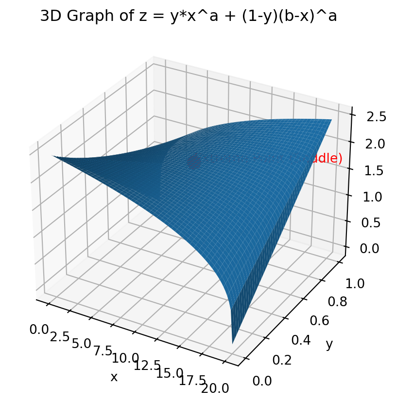
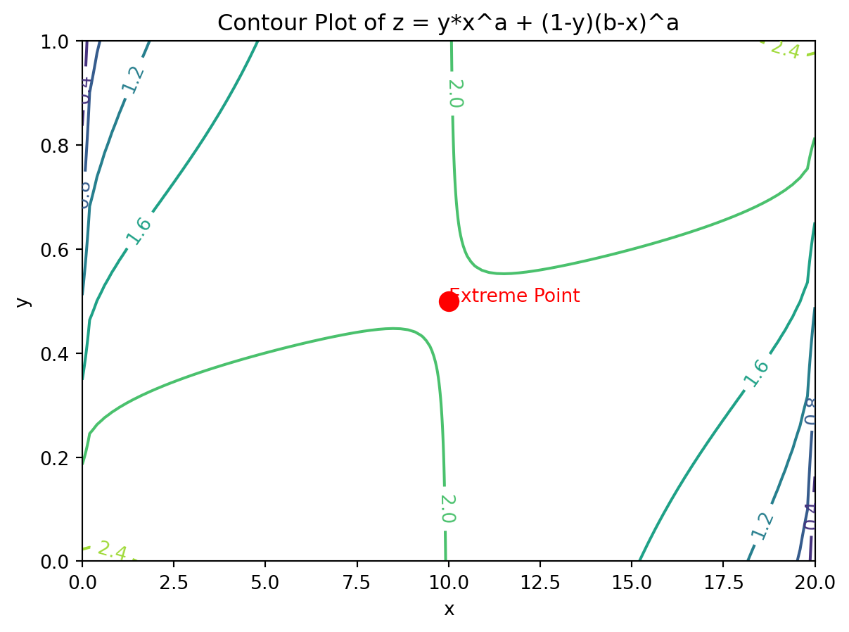
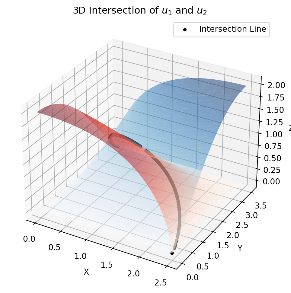
# Define functions u_1(x,y) = x^a * y^(1-a) and u_2(x,y) = (2-x)(2-y)
def u1(x, y):
    return x**(scale*a) * y**(scale*(1-a))

def u2(x, y):
    return (k_x - x)**(scale*a) * (k_y - y)**(scale*(1-a))

# Define the grid
x = np.linspace(0, k_x, 15)
y = np.linspace(0, k_y, 15)
X, Y = np.meshgrid(x, y)

# Compute the numerical derivatives (vector field components)
U1, V1 = numerical_derivative(u1, X, Y)
U2, V2 = numerical_derivative(u2, X, Y)

# Reduce the density of vectors for better visualization
x_sparse = np.linspace(0, k_x, 8)
y_sparse = np.linspace(0, k_y, 8)
X_sparse, Y_sparse = np.meshgrid(x_sparse, y_sparse)
U1_sparse, V1_sparse = numerical_derivative(u1, X_sparse, Y_sparse)
U2_sparse, V2_sparse = numerical_derivative(u2, X_sparse, Y_sparse)

# Plot the combined vector fields and contour plots
#plt.figure(figsize=(8, 8))

# Contour plots of u_1 and u_2 (level curves only)
contour1 = plt.contour(X, Y, u1(X, Y), colors='blue', linestyles='solid', linewidths=1)
contour2 = plt.contour(X, Y, u2(X, Y), colors='red', linestyles='dashed', linewidths=1)

# Overlay vector fields
plt.quiver(X_sparse, Y_sparse, U1_sparse, V1_sparse, color='b', angles='xy', label='∇$u_1$')
plt.quiver(X_sparse, Y_sparse, U2_sparse, V2_sparse, color='r', angles='xy', label='∇$u_2$')

# Labels and grid
plt.xlabel('x')
plt.ylabel('y')
plt.title('Gradient Vector Fields & Level Curves of $u_1$ and $u_2$')
plt.legend()
plt.grid('scaled')
plt.axis('square')

plt.tight_layout()
# Show the plot
plt.show()

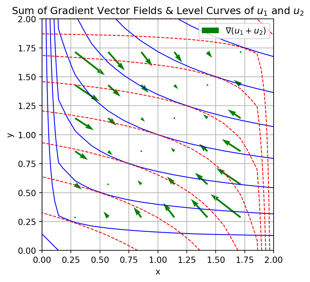
# Compute the sum of gradients
U_sum = U1 + U2
V_sum = V1 + V2

# Reduce the density of vectors for better visualization
U_sum_sparse, V_sum_sparse = numerical_derivative(lambda x, y: u1(x, y) + u2(x, y), X_sparse, Y_sparse)

# Plot the combined vector fields and contour plots
#plt.figure(figsize=(8, 8))

# Contour plots of u_1 and u_2 (level curves only)
contour1 = plt.contour(X, Y, u1(X, Y), colors='blue', linestyles='solid', linewidths=1)
contour2 = plt.contour(X, Y, u2(X, Y), colors='red', linestyles='dashed', linewidths=1)

# Overlay sum of gradient vector fields
plt.quiver(X_sparse, Y_sparse, U_sum_sparse, V_sum_sparse, color='g', angles='xy', label='∇($u_1 + u_2$)')

# Labels and grid
plt.xlabel('x')
plt.ylabel('y')
plt.title('Sum of Gradient Vector Fields & Level Curves of $u_1$ and $u_2$')
plt.legend()

plt.grid('scaled')
plt.axis('square')
# Show the plot
plt.show()

8 Appendix: Sigmoid utility function

import numpy as np
import matplotlib.pyplot as plt
from mpl_toolkits.mplot3d import Axes3D

# Define constants
kx = (np.pi**3 / 2) ** (1/3)
ky = (2**(1/2)) * ((np.pi**3 / 2) ** (1/3))

# Define the grid
x = np.linspace(0, kx, 1000)
y = np.linspace(0, ky, 1000)
X, Y = np.meshgrid(x, y)

# Define the functions
u1 = 1 - np.cos(X**(1/3) * Y**(2/3))
u2 = 1 - np.cos((kx - X)**(1/3) * (ky - Y)**(2/3))

# Find intersection points where u1 == u2
threshold = 1e-3  # Numerical tolerance for equality
intersection_mask = np.abs(u1 - u2) < threshold
X_intersect = X[intersection_mask]
Y_intersect = Y[intersection_mask]
Z_intersect = u1[intersection_mask]  # u1 and u2 are nearly equal

# Create 3D plot
fig = plt.figure(figsize=(8, 6))
ax = fig.add_subplot(111, projection='3d')

# Plot intersection line
ax.scatter(X_intersect, Y_intersect, Z_intersect, color='black', s=10, label='Intersection Line')

# Surface plots for reference
ax.plot_surface(X, Y, u1, cmap='Blues', alpha=0.5)
ax.plot_surface(X, Y, u2, cmap='Reds', alpha=0.5)

# Labels and title
ax.set_xlabel('X')
ax.set_ylabel('Y')
ax.set_zlabel('Z')
ax.set_title('3D Intersection of $u_1$ and $u_2$')
ax.legend()

plt.show()

References

Arrow, Kenneth J., and Gerard Debreu. 1954. “Existence of an Equilibrium for a Competitive Economy.” Econometrica 22 (3): 265–90.

Arthur, W. Brian. 1994. Increasing Returns and Path Dependence in the Economy. University of Michigan Press.

Debreu, Gerard. 1959. Theory of Value: An Axiomatic Analysis of Economic Equilibrium. Yale University Press.

Katz, Michael L., and Carl Shapiro. 1985. “Network Externalities, Competition, and Compatibility.” The American Economic Review 75 (3): 424–40.

Rochet, Jean-Charles, and Jean Tirole. 2003. “Platform Competition in Two-Sided Markets.” Journal of the European Economic Association 1 (4): 990–1029.

Shleifer, Andrei, and Robert W. Vishny. 1993. “Corruption.” The Quarterly Journal of Economics 108 (3): 599–617.

Tirole, Jean. 1988. The Theory of Industrial Organization. MIT Press.