Introduction
This report extends my empirical findings from the ME5 PRIOR research portfolios (of Fama and French) into a broader philosophical and socioeconomic interpretation. I draw connections between large-cap momentum dynamics in capital markets and foundational ideas from ethics, social choice theory, and political philosophy.
The core phenomenon observed—persistent outperformance among firms that are already the largest and most successful—bears striking resemblance to the biblical and sociological concept of the Matthew Effect:
“For to every one who has, more will be given…” — Matthew 25:29
In financial markets, this is not merely a parable—it is measurable, structural, and persistent. It reveals that what appears to be a free, fair, and competitive economy may in fact be a self-reinforcing regime of privilege, cloaked under the language of freedom, equality, fairness, and consent—the founding pillars of liberal democracy.
Structural Inequality at the Firm level
My analysis of the ME5 PRIOR portfolios revealed the following:
- Even within the top 20% of firms by market capitalization (ME5), those that performed best in the prior 11 months (PRIOR5) tend to continue outperforming in the subsequent period.
- This effect is particularly strong post-2010, aligning with macroeconomic changes such as quantitative easing, the rise of passive investing, and capital concentration.
- This implies a reinforcing feedback loop: prior success draws more capital, more capital enables further success, and performance becomes increasingly decoupled from diversification.
The analogy to social mobility is immediate: those who have, get more—not just relatively, but absolutely and increasingly.
The Matthew Effect at the Household Level
If capital lock-in dynamics operate not only at the firm level but also across households—a plausible and empirically supported assumption—the implications are far-reaching:
- Wealthy households benefit disproportionately from capital gains and passive income
- Lower- and middle-income households rely predominantly on labor income, with limited upside
- The result is a declining probability of upward mobility, and increasing wealth stratification
This structure undermines the ideal of a meritocratic liberal democracy where opportunity is equitably distributed and fairness is institutionalized. In reality, the capital system begins to resemble a rigged equilibrium, where the initial balance is illusionary—a symbolic counterweight with no real effect.
The Philosophical Lens: Arrow, Spinoza, and Pascal
Arrow’s utilitarian social welfare framework assumes at least some degree of fairness and fluidity among agents. But in a setting of structural inequality and declining mobility:
- The expected utility of society does not necessarily increase, even if total capital grows
- The bottom half of society may experience static or declining utility, overwhelmed by the persistent rise of the elite
From a Spinozist viewpoint, this is a failure of a rational, self-sustaining society—it lacks balance and cohesion. For Pascal, it raises the existential irony of a system designed for all, yet serving few.
And if we apply Rawls’ difference principle, we see an institutional failure to justify inequality based on benefit to the least advantaged. Liberal democracy, viewed from the perspective of financial capitalism, begins to fracture: the ideals of liberty, fairness, and equality become ceremonial rather than structural.
Conclusion
The Matthew Effect is not just a biblical principle—it is a lived, structural condition of our financial and social reality.
The capital markets amplify this dynamic, and unless counterbalanced by social, policy, or philosophical intervention, it threatens not only equity, but long-term stability and collective welfare.
Appendix: ME5 PRIOR Portfolios
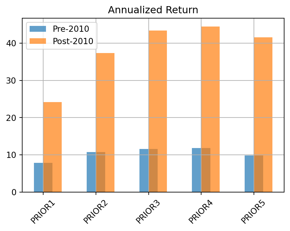
In this report, I examined the persistence of momentum within the top market-cap group (ME5) using the Fama-French 25 Portfolios sorted by size and prior return. Specifically, I analyzed how the performance of five portfolios (PRIOR1 to PRIOR5), sorted by prior 11-month returns within the ME5 group, has evolved between two distinct market regimes: pre-2010 and post-2010.
The results are striking.
Even among the largest companies (top 20% by market cap), those that performed best over the prior year continued to outperform in the next month—both in the pre and post-2010 market regime.
What initially seemed like a behavioral or statistical curiosity turns out to reflect a deeper transformation of the market’s internal structure—a transformation where capital flows, visibility, and narrative dominance now reinforce past winners among the already-rich. In this setting, the language of freedom, fairness, and opportunity—so essential to liberal democracy—becomes less about equal access and more about locked-in advantage. The market becomes a mirror, not of fair competition, but of Matthew Effect dynamics, where “to those who have, more shall be given.”
For risk-aware investors engaged in short-term, monthly rebalancing, the implications are concrete:
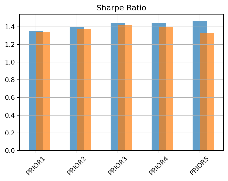
- PRIOR3 offers exceptional consistency with lower volatility and downside exposure
- PRIOR5 delivers superior absolute return with tolerable risk
- Both are based on highly liquid, mega-cap stocks, making them operationally feasible and institutionally scalable
In short: Even among the richest firms, past winners tend to keep winning.
Momentum is no longer a temporary anomaly. It is part of the architecture.
This realization challenges equilibrium-based pricing models and calls into question our normative assumptions about economic fairness. If capital accumulates in a non-reverting way among the already-powerful, mobility collapses—and with it, the utilitarian social welfare that undergirds Arrow’s idealized world of dynamic fairness. What remains is a hollow pendulum: a financial system that swings, but never truly balances.
Methodology
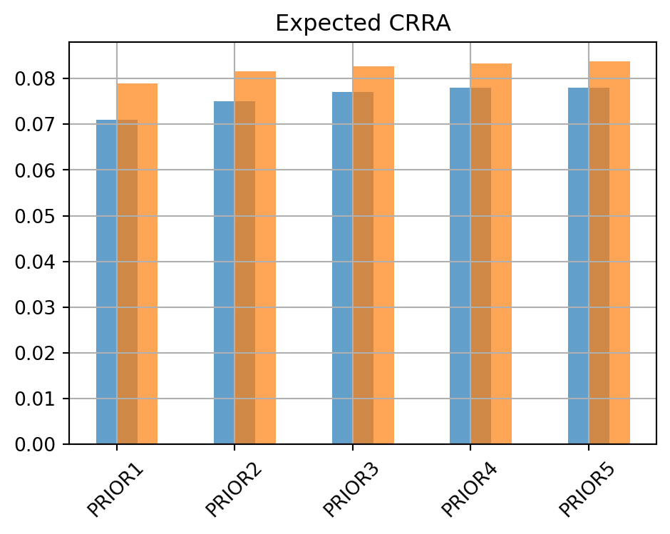
We compute a comprehensive set of performance metrics (e.g., annualized return, Sharpe, Sortino, Calmar, Omega, expected CRRA utility) for each ME5 PRIOR portfolio across two structural periods:
- Pre-2010: January 1996 to December 2009
- Post-2010: January 2010 to December 2023
All returns are monthly and expressed as decimals (net of compounding). Metrics are calculated for value-weighted portfolios of NYSE-listed firms within ME5, using prior 11-month cumulative returns (excluding the most recent month) to define momentum quintiles.
Empirical Summary and Interpretation
- Pre-2010:
- PRIOR5 was most effective for risk-adjusted returns (e.g. Sharpe , Sortino)
- PRIOR4 had higher return, but more volatility and negative skew
- PRIOR1 severely underperformed (negative average return, deep drawdowns)
- Post-2010:
- Momentum dominance continued
- PRIOR4 exhibits top raw returns and Sortino.
- Both dominate the risk-return landscape with resilience and predictability
The market is no longer cyclical, but directional; no longer egalitarian, but reinforcing. Passive capital flows, QE-induced yield suppression, and index-based exposure collectively sustain a regime where “winners win more, losers lag longer.” If the ideal of equal opportunity was once the balancing pendulum of a free market society, the modern financial system now swings in only one direction.